11 Chemical Equilibrium and Mixtures
Part IV — Phase Transitions and Chemical Equilibrium
Last updated: 14-07-2026
11.1 Where this lecture is going
Mix nitrogen and hydrogen in given proportions and let them react: ammonia forms, but the reaction stops partway. A definite fraction of the mixture converts, the same every time the experiment is repeated at the same temperature and pressure, larger when the mixture is compressed, smaller when it is heated. Nothing in the stoichiometry hints at a stopping point: the equation \(\mathrm{N_2 + 3H_2 \rightleftharpoons 2NH_3}\) would happily run until a reactant is exhausted. Two questions run through this lecture: where does a reacting mixture come to rest, and how does the resting point move when the pressure or the temperature is changed?
The machinery is in place. At fixed \(T\) and \(p\) a system settles where its Gibbs free energy is least (Equation 10.6), and Lecture 10 reduced this, for a reacting mixture, to the condition \(\sum_i \nu_i \mu_i = 0\) on the chemical potentials. What that lecture could not say is which composition the condition selects, because the chemical potentials of a mixture depend on the composition, and that dependence had not yet been computed. Computing it is the opening business of this lecture. For a mixture of ideal gases it is the logarithmic law promised in Lecture 8: each component obeys Equation 8.9 with its own partial pressure in place of the pressure. The logarithm is the entropy of mixing at work, and it settles half of the first question by itself: it makes the Gibbs free energy descend steeply wherever a species is about to vanish, so the minimum lies strictly inside the reaction interval, and no reaction runs to completion. Where inside, the same law answers once it is fed into the equilibrium condition: it becomes the law of mass action, which condenses the equilibrium composition of any reacting ideal mixture into a single number per reaction and temperature. Half of the second question is then read off the law directly: compression shifts the equilibrium toward the side with fewer moles of gas, the compression half of the ammonia opening. The other half, the response to the temperature, acts through the equilibrium constant itself and is developed in a closing supplementary section, left to reading.
Throughout, the system is a single homogeneous phase of several ideal gases: molecules so dilute that they do not interact, the one case in which the chemical potentials take an explicit form. The general framework of phases, species and reactions built in Lecture 10 is inherited and cited, not re-derived; mixtures of liquids, and solutions, lie outside the scope of this course.
The path: first the mixture relations and the multicomponent Gibbs–Duhem relation; then the ideal gas mixture, with Dalton’s law, the entropy of mixing and the chemical potentials; then the Gibbs free energy along a reaction and its interior minimum; the law of mass action, worked in full for one dissociation; and the effect of pressure, which answers the compression half of the ammonia opening. The heating half is the supplementary reading.
11.2 Mixtures and the multicomponent Gibbs–Duhem relation
Everything in this lecture happens inside a single homogeneous body carrying several species: a mixture, one phase in the language of Lecture 10. Its thermodynamics is already in hand, proved there for a phase of any composition, and it carries over unchanged with the phase index dropped. Writing \(n_i\) for the amount of species \(i = 1, \dots, N_s\), the fundamental relation Equation 10.1 reads \[ dU = T\,dS - p\,dV + \sum_i \mu_i\,dn_i, \] with \(\mu_i\) the chemical potential of species \(i\) in the mixture; extensivity forces the Euler relation Equation 10.2, \[ U = TS - pV + \sum_i \mu_i\,n_i ; \] and the Gibbs free energy \(G = U - TS + pV\) carries the differential Equation 10.3 and the value Equation 10.4, \[ dG = -S\,dT + V\,dp + \sum_i \mu_i\,dn_i, \qquad G = \sum_i n_i\,\mu_i, \] with \(\mu_i = (\partial G/\partial n_i)_{T,p,\,n_{j\neq i}}\) the partial molar Gibbs free energy of species \(i\).
Mixture — a single homogeneous phase containing several species; its composition is part of its state.
One consequence was not needed in that lecture and we draw it now, by the step used for one component in Lecture 9. The Euler relation holds identically, so its differential must agree with the fundamental relation; and since it expresses the internal energy through the intensive variables \(T\), \(p\) and \(\mu_i\) as well as the extensive \(S\), \(V\) and \(n_i\), its differential carries their increments too, \[ dU = T\,dS + S\,dT - p\,dV - V\,dp + \sum_i \mu_i\,dn_i + \sum_i n_i\,d\mu_i . \] Subtracting the fundamental relation leaves the multicomponent Gibbs–Duhem relation \[ S\,dT - V\,dp + \sum_i n_i\,d\mu_i = 0 . \tag{11.1}\] For a single species it is the relation Equation 9.4 of Lecture 9. Its content, as there, is that the intensive variables are not all independent. New is its reading at fixed temperature and pressure, where it becomes \(\sum_i n_i\,d\mu_i = 0\): however the composition of a mixture is changed at given \(T\) and \(p\), the chemical potentials cannot all rise or all fall together; a change that raises some must lower others, weighted by the amounts present. The relation will also serve, later in the next section, as a consistency check on the chemical potentials of the ideal gas mixture.
Multicomponent Gibbs–Duhem \(S\,dT - V\,dp + \sum_i n_i\,d\mu_i = 0\) — at fixed \(T\) and \(p\) the chemical potentials of a mixture cannot change independently: \(\sum_i n_i\,d\mu_i = 0\).
What can the chemical potentials depend on? The Gibbs free energy is extensive, and its only extensive arguments are the amounts: the temperature and the pressure are intensive, untouched when the body is scaled. Extensivity therefore reads \(G(T, p, \{\lambda n_j\}) = \lambda\,G(T, p, \{n_j\})\), the scaling that gave \(G = \mu n\) for one component in Lecture 9, now with several amounts. Differentiating both sides with respect to \(n_i\), the left through the chain rule, and cancelling the common factor \(\lambda\) gives \[ \mu_i(T, p, \{\lambda n_j\}) = \mu_i(T, p, \{n_j\}) : \] the chemical potentials are unchanged when the mixture is scaled up, so they depend on the amounts only through their ratios. We measure the ratios against the total amount \(n = \sum_j n_j\), defining the mole fractions \[ x_i = \frac{n_i}{n}, \qquad \sum_i x_i = 1, \] of which \(N_s - 1\) are independent. (The symbol repeats that of the lever rule of Lecture 10, where it counted the fraction of matter in each phase; here \(x_i\) is the fraction of each species within the one phase.) Each chemical potential is therefore a function \(\mu_i(T, p, x_1, \dots, x_{N_s - 1})\) of the temperature, the pressure and the composition.
Mole fraction \(x_i = n_i/n\) — the composition variables of a mixture; they sum to one, so \(N_s - 1\) are independent.
For one component the list of composition variables is empty and the chemical potential is a function of \(T\) and \(p\) alone, as the Gibbs–Duhem relation forced in Lecture 9; adding matter at fixed temperature and pressure then merely makes more of the same, \((\partial\mu/\partial n)_{T,p} = 0\), as discussed in Lecture 8 and Problem 8.12. In a mixture the composition is a genuine freedom, and the count matches the phase rule Equation 10.9: one phase of \(N_s\) non-reacting species has \(f = N_s - 1 + 2 = N_s + 1\) intensive variables, the temperature, the pressure and the \(N_s - 1\) mole fractions. The dependence of the chemical potentials on the composition is the one piece of the theory not yet computed; the next section computes it in the one case where it takes an explicit form, the ideal gas mixture.
11.3 The ideal gas mixture
The one mixture whose chemical potentials we can compute explicitly is built from the ideal gas. Lecture 4 defined it empirically, as the low-density limit that every real gas approaches; the molecular reading of that limit came with the energy equation of Lecture 9, whose internal pressure, the energy cost of drawing the molecules apart, vanishes for the ideal gas: the molecules do not interact. At such densities, molecules of different species meet as rarely as molecules of the same one. This suggests the picture behind the ideal gas mixture: no molecule interacts with any other, whatever its species, so each species is unaffected by the presence of the rest and behaves as if it occupied the vessel alone. Alone in the volume \(V\) at temperature \(T\), species \(i\) would exert the pressure \(p_i = n_i RT/V\), its partial pressure; the pressure of the mixture is the sum of these non-interacting contributions, \[ p = \sum_i p_i = \frac{nRT}{V} , \qquad p_i = x_i\,p , \tag{11.2}\] Dalton’s law. The mixture as a whole thus obeys the ideal-gas equation of state with the total amount \(n\), and each partial pressure is the total pressure weighted by the mole fraction, since \(p_i/p = n_i/n\).
Partial pressure \(p_i = n_i RT/V\) — the pressure species \(i\) would exert alone in the vessel; well defined only in the dilute limit.
Dalton’s law \(p = \sum_i p_i\) — the partial pressures of an ideal mixture add up to the measured pressure.
A word of caution before the concept is put to work: the partial pressure is well defined only within the dilute-gas idealisation. When the molecules do not interact, each species strikes the walls exactly as it would alone, and “the pressure species \(i\) would exert alone in the vessel” is a physically meaningful decomposition of the measured \(p\), the contributions adding as in Equation 11.2. In a dense gas the force on the walls is produced by all the molecules and their mutual interactions together, and no part of it can be attributed to one species; the product \(x_i\,p\) can always be written down, but there it is a bookkeeping definition, not a pressure that anything exerts.
The same reading fixes the state functions. The internal energy is the sum of what each species would have alone, \(U = \sum_i n_i\,u_i(T)\), each molar energy \(u_i\) a function of the temperature alone (Lecture 4); and the entropy likewise, \[ S(T, V, \{n_j\}) = \sum_i S_i(T, V, n_i), \] each summand the ideal-gas entropy Equation 8.5 that species \(i\) would have alone in the vessel. The two statements do not have the same standing. The pressure and the energy are mechanical, and that non-interacting molecules strike the walls and store energy independently is the direct content of the molecular picture. Nothing, however, fixes from first principles how the entropy depends on the composition: its additivity is a genuine further assertion, and it is this that we take as the definition of the ideal gas mixture, the molecular picture serving as motivation. Its consequences are checked below, against the Gibbs–Duhem relation and, through the law of mass action, against experiment.
With the entropy in hand, the first consequence is the entropy cost of mixing itself. Let two different gases occupy adjoining compartments of a rigid, isolated vessel, \(n_1\) moles in the volume \(V_1\) and \(n_2\) in \(V_2\), both at the same temperature \(T\) and pressure \(p\), and let the partition be removed (Figure 11.1). The gases interdiffuse until the mixture is uniform over \(V = V_1 + V_2\). No heat enters and no work is done, so \(U\) is unchanged; since \(U = \sum_i n_i u_i(T)\) depends on the state only through \(T\), the temperature is unchanged too, and with it the pressure, \(p = nRT/V\). The entropy, additive over the two bodies before (Lecture 6) and over the two species after, changes only through the volume argument of each term, exactly as in the free expansion of Lecture 7: \[ \Delta S_{\rm mix} = \sum_i \big[ S_i(T, V, n_i) - S_i(T, V_i, n_i) \big] = \sum_i n_i R \ln\frac{V}{V_i} . \] At the common \(T\) and \(p\) the volumes stand in the ratio of the amounts, \(V_i/V = x_i\), so, writing \(n_i = n x_i\), the entropy of mixing is \[ \Delta S_{\rm mix} = \sum_i n_i R \ln\frac{1}{x_i} = -\,nR \sum_i x_i \ln x_i \; > \; 0 , \tag{11.3}\] positive because every \(x_i < 1\), and valid as it stands for any number of species. Each gas has, in effect, expanded freely into the volume held by the other; nothing else in the universe has changed, so the mixing of gases is irreversible and raises the total entropy, the remaining example promised in Lecture 7. The scale is the usual \(R\): for two equimolar gases, \(\Delta S_{\rm mix} = nR\ln 2\), about \(5.8\ \mathrm{J\,K^{-1}}\) per mole of mixture.
Entropy of mixing \(\Delta S_{\rm mix} = -nR\sum_i x_i \ln x_i\) — the entropy created when gases at the same \(T\) and \(p\) interdiffuse; irreversible.
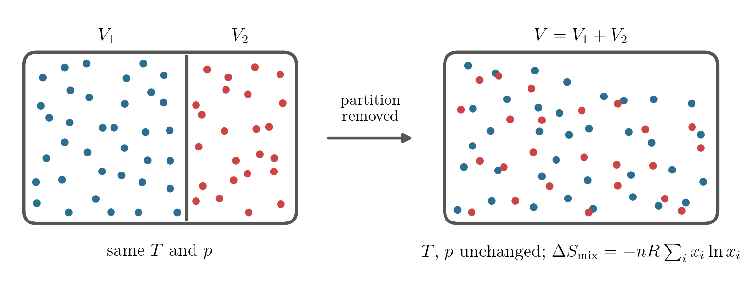
The entropy of mixing Equation 11.3 does not depend on the nature of the gases: nitrogen interdiffusing with oxygen or with argon produces the same \(\Delta S_{\rm mix}\), however alike the two species, provided they are distinct. If instead the two compartments hold one and the same gas, the entropy change vanishes. That is a computation, not an appeal to intuition: at the common \(T\) and \(p\) the molar volume \(v = V_1/n_1 = V_2/n_2 = V/n\) is the same in each compartment and in the whole vessel, so the additivity of the entropy over the two bodies (Lecture 6) and its extensivity give \[ S_{\rm initial} = n_1\,s(T, v) + n_2\,s(T, v) = n\,s(T, v) = S_{\rm final} . \]
The paradox is the discontinuity. One might expect the mixing entropy to fade gradually as the two species are imagined more and more alike, vanishing in the limit; instead it keeps the full value \(-nR\sum_i x_i \ln x_i\) for every pair of distinct species and equals zero for identical ones, with nothing in between. The resolution is that \(\Delta S\) compares states, and the two cases compare different pairs of states. For distinct species the unmixed and the mixed configurations are distinct equilibrium states: some physical process separates any two distinct species (condensation at their different boiling points, selective absorption, a wall permeable to one species and not the other), so the unmixed state can be restored at the same temperature, and by the free-energy bound Equation 9.11 that restoration costs at least the work \(T\,\Delta S_{\rm mix}\). For a single species the “unmixed” and “mixed” configurations are one and the same equilibrium state, described by the same \((T, V, n)\), and there is nothing to restore. Thermodynamics therefore treats the distinctness of species as an all-or-nothing property; no measure of similarity appears anywhere in the theory. How this squares with the continuously variable parameters of molecular physics is answered by the quantum theory of identical particles, in statistical mechanics.
The chemical potential of a component follows most directly from the Helmholtz free energy, because its natural variables \(T\), \(V\) and the amounts are exactly the variables in which the species decouple. The Legendre step of Lecture 9 applied to the fundamental relation of the mixture gives \(dF = -S\,dT - p\,dV + \sum_i \mu_i\,dn_i\), so that \(\mu_i = (\partial F/\partial n_i)_{T,V,\,n_{j\neq i}}\), the same chemical potential read off a different potential. And at fixed \(T\) and \(V\) the Helmholtz free energy of the mixture falls apart into pure-gas pieces: \[ F = U - TS = \sum_i \big[ n_i\,u_i(T) - T\,S_i(T, V, n_i) \big] = \sum_i F_i(T, V, n_i), \] each term the Helmholtz free energy that pure gas \(i\) would have alone in the vessel. The derivative with respect to \(n_i\) touches a single term, and \((\partial F_i/\partial n_i)_{T,V}\) is precisely the chemical potential of the pure ideal gas computed in Lecture 8, a function of the temperature and of the molar volume \(V/n_i\) at which the species sits. A pure gas at that temperature and molar volume has the pressure \(n_i RT/V\), which is the partial pressure \(p_i\); so the derivative is the pure gas’s chemical potential taken at \((T, p_i)\). Writing \(\mu_i^{\rm pure}(T, p)\) for the pure-gas function Equation 8.9 of species \(i\), we have found \[ \mu_i = \mu_i^{\rm pure}(T, p_i) = \mu_i^{\rm pure}(T, p_0) + RT \ln\frac{p_i}{p_0} : \tag{11.4}\] the chemical potential of a component of an ideal gas mixture is that of the pure gas at the same temperature and its own partial pressure. This is Equation 8.9 with \(p\) replaced by \(p_i\), exactly the form Lecture 8 promised. From here on the unadorned \(\mu_i\) always denotes the component in the mixture, and the superscript marks the pure-gas function.
Chemical potential of a component \(\mu_i = \mu_i^{\rm pure}(T, p_i)\) — the pure gas’s chemical potential at the same \(T\) and its own partial pressure \(p_i\).
The last three lectures worked almost exclusively with the Gibbs free energy, and reaching now for \(F\) may look like a change of framework. It is not. The four potentials of Lecture 9 carry the same information: each is obtained from any other by a Legendre transform, and the transform loses nothing (from \(F\), for instance, \(S = -(\partial F/\partial T)_{V,n}\) recovers \(U = F + TS\)), so any one of them determines the full thermodynamics of the system. In particular the chemical potential of a species is the coefficient of \(dn_i\) in all four differentials at once, as noted for one component in Lecture 9: \[ \mu_i = \left(\frac{\partial U}{\partial n_i}\right)_{S,V} = \left(\frac{\partial H}{\partial n_i}\right)_{S,p} = \left(\frac{\partial F}{\partial n_i}\right)_{T,V} = \left(\frac{\partial G}{\partial n_i}\right)_{T,p}, \] the other amounts held fixed in each. Which derivative to evaluate is purely a question of convenience: one picks the potential whose natural variables match the structure of the problem at hand. In Lecture 10 that was \(G\), because phases exchange matter at a common temperature and pressure, the variables \(G\) holds naturally. Here the structure to exploit is the decoupling of the species, and the species share the vessel, not the pressure: at fixed \(T\) and \(V\) the Helmholtz free energy of the mixture is a sum of pure-gas terms, one per species, while at fixed \(T\) and \(p\) the Gibbs free energy is not, since changing \(n_i\) at fixed total pressure shifts every partial pressure \(p_j = x_j p\), and the species stay coupled through the composition. Differentiating \(G\) yields the same \(\mu_i\), but only after a sum of cross terms cancels (an instructive check, taken up in the problems); differentiating \(F\) touches a single term. The result is the same either way, as it must be.
Splitting the partial pressure as \(p_i = x_i p\) (Equation 11.2) and absorbing the \(RT\ln(p/p_0)\) into the pure-gas value at the total pressure puts the same result in the form \[ \mu_i = \mu_i^{\rm pure}(T, p) + RT \ln x_i , \tag{11.5}\] which compares the component directly with the pure gas at the same \(T\) and the same total \(p\). Since \(\ln x_i < 0\), mixing lowers every chemical potential: each species is worth less, per mole, inside the mixture than pure at the same temperature and pressure. The reading is the one established in Lecture 8: matter flows toward low chemical potential, so a pure gas brought into contact with a mixture at the same \(T\) and \(p\) flows into it, and gases interdiffuse spontaneously. The same fact in the Gibbs free energy: from \(G = \sum_i n_i \mu_i\) (Equation 10.4), mixing at fixed \(T\) and \(p\) changes \(G\) by \(\sum_i n_i RT \ln x_i = -T\,\Delta S_{\rm mix} < 0\), downhill exactly as the minimum principle Equation 9.12 requires. And the multicomponent Gibbs–Duhem relation is satisfied, as promised: at fixed \(T\) and \(p\), using \(n_i = n x_i\), \[ \sum_i n_i\,d\mu_i = RT \sum_i n_i\,\frac{dx_i}{x_i} = nRT\,\sum_i dx_i = 0 , \] since the mole fractions sum to one (Equation 11.1).
One more consequence settles the question left open in Problem 8.12. At fixed \(T\) and \(p\) the chemical potential of a component depends on its own amount through \(x_i\) alone. Differentiating \(x_i = n_i/n\), with the total \(n = \sum_j n_j\) carrying its own \(n_i\), gives \((\partial x_i/\partial n_i)_{n_{j\neq i}} = (1 - x_i)/n\), so Equation 11.5 yields \[ \left(\frac{\partial \mu_i}{\partial n_i}\right)_{T,p,\,n_{j\neq i}} = RT\,\frac{1 - x_i}{n_i} \; > \; 0 : \] adding a species to a mixture raises that species’ own chemical potential. This is the diffusive stability condition that the one-component system could not have, where \((\partial\mu/\partial n)_{T,p} = 0\) identically: in a mixture the composition is a genuine thermodynamic direction, and it is a stable one.
11.4 The Gibbs free energy along a reaction
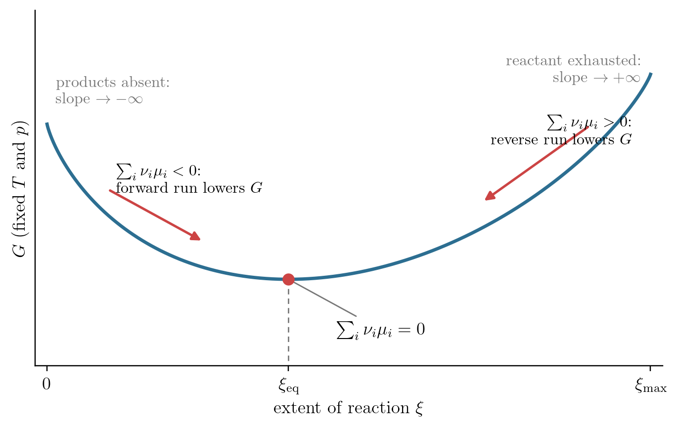
Now let the species react. That the molecules of an ideal mixture do not interact is no obstacle: encounters rare enough to leave the state functions untouched still occur, and they, or a catalyst, are the channel through which matter passes from one species to another. Thermodynamics fixes where the composition comes to rest, not how fast it gets there. The kinematics was set out in Lecture 10: a reaction consumes and produces species in fixed whole-number proportions, its stoichiometric coefficients \(\nu_i\), counted negative for a species consumed and positive for one produced, and it advances by a single number, its extent \(\xi\), every amount changing in lockstep as \(dn_i = \nu_i\,d\xi\). For the ammonia synthesis of the opening, \(\mathrm{N_2 + 3H_2 \rightleftharpoons 2NH_3}\), the coefficients are \((\nu_{\mathrm{N_2}}, \nu_{\mathrm{H_2}}, \nu_{\mathrm{NH_3}}) = (-1, -3, +2)\). Let the mixture now be held at the temperature and pressure of its surroundings, in the arrangement of Lecture 10: the vessel is closed, so the amounts change through the reaction alone, \(n_i(\xi) = n_i^0 + \nu_i\,\xi\), with \(\xi\) confined to the interval on which every \(n_i \ge 0\). At fixed \(T\) and \(p\) the Gibbs free energy is then a function of the one variable \(\xi\), and its slope follows from \(dG = \sum_i \mu_i\,dn_i\) (Equation 10.7): \[ \left(\frac{\partial G}{\partial \xi}\right)_{T,p} = \sum_i \nu_i\,\mu_i , \tag{11.6}\] the chemical potentials evaluated at the composition the mixture has reached, exactly as in Lecture 10; since the \(\mu_i\) move with the composition, the slope varies along the way and \(G(\xi)\) traces out a curve.
Slope of \(G\) along a reaction \((\partial G/\partial\xi)_{T,p} = \sum_i \nu_i \mu_i\) — negative where the forward run lowers \(G\), zero at equilibrium.
The second law reads this slope. At fixed \(T\) and \(p\) a spontaneous change can only lower the Gibbs free energy (Equation 10.6), so the reaction runs in the direction of descending \(G\): forward where \(\sum_i \nu_i \mu_i < 0\), in reverse where it is positive, and to rest where the slope vanishes, \[ \sum_i \nu_i\,\mu_i = 0 , \] the reaction-equilibrium condition named in Lecture 10. The sum weighs, mole for mole, the chemical potential of what appears against that of what disappears: the reaction transfers matter from the side of higher total chemical potential to the lower, the same downhill flow in \(\mu\) established in Lecture 8, running here through the composition rather than through space.
Whether the rest point lies at an end of the interval, meaning complete conversion, or inside it is decided by the mixing term \(RT\ln x_i\) of Equation 11.5, which sends \(\mu_i \to -\infty\) as \(x_i \to 0\). At either end of the interval the amount of some species vanishes, and an advance from that end into the interval regenerates the species from nothing; the term \(RT \ln x_i\) then lowers \(G\) steeply, however unfavourable the pure-gas value \(\mu_i^{\rm pure}\). Concretely, starting from pure reactants the products are absent, each product term \(\nu_i \mu_i\) of Equation 11.6 tends to \(-\infty\), and the first advance of the reaction lowers \(G\) with unbounded slope; approaching complete conversion the exhausted reactant is the vanishing species, its term (with \(\nu_i < 0\)) tends to \(+\infty\), and converting its last trace raises \(G\) with unbounded slope. The Gibbs free energy therefore descends into the interval from both ends, and its minimum lies strictly inside (Figure 11.2). The physics behind the logarithm is the entropy of mixing: the first traces of an absent species carry a large entropy gain at negligible cost, so keeping a little of everything always lowers \(G\). Hence no reaction runs to completion: at equilibrium every species is present, if need be in traces. The contrast with phase coexistence is worth drawing. Between two coexisting phases the Gibbs free energy is flat along the transfer of matter (\(\mu_1 = \mu_2\), so moving \(dn\) across changes nothing), which is why Lecture 10 found the split between the phases undetermined, left to the surroundings to set; along a reaction the mixing entropy curves \(G(\xi)\) and pins a unique equilibrium composition. This answers the first question of the opening; where exactly the minimum falls is computed in the next section.
No reaction runs to completion — the mixing entropy makes the minimum of \(G(\xi)\) interior; every species survives at equilibrium, possibly in traces.
11.5 The law of mass action
The equilibrium condition \(\sum_i \nu_i \mu_i = 0\) becomes explicit the moment the chemical potentials of the ideal mixture are inserted. With Equation 11.4, \[ \sum_i \nu_i\,\mu_i^{\rm pure}(T, p_0) + RT \sum_i \nu_i \ln\frac{p_i}{p_0} = 0 , \] and the logarithms gather into one, \(\sum_i \nu_i \ln(p_i/p_0) = \ln \prod_i (p_i/p_0)^{\nu_i}\). Solving for the product, \[ \prod_i \left(\frac{p_i}{p_0}\right)^{\nu_i} = K(T) , \qquad K(T) = \exp\left[-\,\frac{\sum_i \nu_i\,\mu_i^{\rm pure}(T, p_0)}{RT}\right] , \tag{11.7}\] the law of mass action. On the left stand the partial pressures of the equilibrium mixture; on the right, the equilibrium constant \(K(T)\), a positive dimensionless number built entirely from the chemical potentials of the pure gases at the reference pressure, and therefore a function of the temperature alone. The number carries the bookkeeping conventions, the choice of \(p_0\) and the overall scale of the \(\nu_i\) (doubling every coefficient squares \(K\)), but the equilibrium compositions it selects do not; a problem makes this precise.
Law of mass action \(\prod_i (p_i/p_0)^{\nu_i} = K(T)\) — the equilibrium composition of any reacting ideal mixture, fixed by one number per reaction and temperature, a property of the pure gases.
The division of labour deserves a pause. The left-hand side is a property of the mixture, as many variables as there are species; the right-hand side never refers to the mixture at all. Everything thermodynamics has to say about the equilibrium composition of an arbitrary reacting mixture, at any proportions of starting materials, is condensed into one number per reaction and temperature, fixed by the pure substances alone. One caveat keeps us honest: to compute \(K\) from thermal measurements on the pure gases one would need their entropy constants, which the course has left open and which only the Third Law supplies (Lecture 12); until then the cleanest measurement of \(K\) is the equilibrium composition itself. The structure of the product carries the signs of the \(\nu_i\): species produced enter upstairs, species consumed downstairs, so a large \(K\) describes a reaction that runs far forward before resting and a small \(K\) one that barely starts; in either case the interior minimum of the last section guarantees that “far” never means “to completion”.
How large is \(K\) typically? The energies freed or bound in chemical transformations are of the order of \(10^2\ \mathrm{kJ\,mol^{-1}}\), while \(RT \approx 2.5\ \mathrm{kJ\,mol^{-1}}\) at room temperature (Lecture 8), so the exponent in Equation 11.7 is typically of order \(\pm 40\) and \(K\) of order \(10^{\pm 17}\). Such an equilibrium sits so close to an end of the reaction interval that the reaction looks complete, or looks as if it had never started: the traces guaranteed by the interior minimum are real but far below anything visible. This is how the law of mass action coexists with the everyday impression that hydrogen burns to the last molecule. The dissociation worked out below is the opposite, and therefore instructive, case: its \(K\) is of order one, the two sides balanced to within a couple of \(RT\), and the interior equilibrium becomes visible.
Worked example: the dissociation of dinitrogen tetroxide. The smallest reacting mixture obeys \(\mathrm{N_2O_4 \rightleftharpoons 2\,NO_2}\), with \((\nu_{\mathrm{N_2O_4}}, \nu_{\mathrm{NO_2}}) = (-1, +2)\). Start from \(n\) moles of pure \(\mathrm{N_2O_4}\) and write \(\alpha\) for its degree of dissociation, the fraction of the initial amount that has split: the mixture holds \(n(1-\alpha)\) moles of \(\mathrm{N_2O_4}\) and \(2n\alpha\) of \(\mathrm{NO_2}\), a total of \(n(1+\alpha)\), so the mole fractions are \[ x_{\mathrm{N_2O_4}} = \frac{1-\alpha}{1+\alpha}, \qquad x_{\mathrm{NO_2}} = \frac{2\alpha}{1+\alpha} . \]
Degree of dissociation \(\alpha\) — the fraction of the initial amount that has split; \(0 \le \alpha \le 1\).
With \(p_i = x_i p\) (Equation 11.2) the law of mass action Equation 11.7 reads \[ K = \frac{(p_{\mathrm{NO_2}}/p_0)^2}{p_{\mathrm{N_2O_4}}/p_0} = \frac{x_{\mathrm{NO_2}}^2}{x_{\mathrm{N_2O_4}}}\,\frac{p}{p_0} = \frac{4\alpha^2}{1-\alpha^2}\,\frac{p}{p_0} , \] which solves in closed form: \[ \alpha = \sqrt{\frac{K}{K + 4\,p/p_0}} . \] At room temperature, \(T = 298\ \mathrm{K}\), the measured constant is \(K \approx 0.15\) (for \(p_0 = 1\ \mathrm{bar}\)); at \(p = 1\ \mathrm{bar}\) this gives \(\alpha \approx 0.19\), about one molecule in five dissociated, an equilibrium sitting squarely in the interior of the reaction interval, as the last section said it must. The composition is visible: \(\mathrm{NO_2}\) is brown and \(\mathrm{N_2O_4}\) colourless, so the depth of colour of the sealed tube displays \(\alpha\), and through it \(K\), to the eye. The ammonia synthesis promised in Problem 10.8 obeys the same law; its composition equation is a quartic in the extent (collapsing to a quadratic for the stoichiometric feed), worked out in the problems. The effect of pressure, however, can be read off without solving anything, and is the subject of the next section.
11.6 Shifting the equilibrium with pressure
The equilibrium constant is a function of the temperature alone, yet the composition it determines does respond to pressure, because the partial pressures carry the total \(p\) inside them. Writing \(p_i = x_i p\) (Equation 11.2) in the law of mass action Equation 11.7 and collecting the factors of \(p\), \[ \prod_i x_i^{\nu_i} = K(T)\left(\frac{p}{p_0}\right)^{-\sum_i \nu_i} : \tag{11.8}\] the mole-fraction product responds to the pressure through the single power \(-\sum_i \nu_i\), the net change in the moles of gas as the reaction advances.
Which way the composition complies is read off the slope of \(G\). Hold the composition fixed for a moment and raise the pressure by \(dp\): by Equation 11.4 every chemical potential grows by the same \(RT\,dp/p\), since only the total pressure moves and the mole fractions do not, so the slope Equation 11.6 changes by \(\left(\sum_i \nu_i\right) RT\,dp/p\). At the old equilibrium the slope was zero; if the reaction increases the amount of gas, \(\sum_i \nu_i > 0\), the slope is now positive, and \(G\) descends toward smaller \(\xi\): the equilibrium moves backward. If the reaction decreases the amount of gas, the slope turns negative and the equilibrium moves forward. In both cases compression drives the equilibrium toward the side with fewer moles of gas. The physical sense is plain: at given \(T\) and \(p\) fewer moles occupy less volume, so the shift is the one that lets the mixture contract under the imposed pressure. The equilibrium answers the disturbance in the sense that opposes it: Le Chatelier’s principle, met in Lecture 8 as the physical reading of stability, here at work on the composition.
Pressure shift — compression at fixed \(T\) moves the equilibrium toward the side with fewer moles of gas (Equation 11.8); the composition shifts so that the mixture yields volume.
The two reactions before us sit on opposite sides of this rule. The ammonia synthesis consumes four moles of gas to make two, \(\sum_i \nu_i = -2\), so compression favours the product, and the factor is large: whatever the value of \(K(T)\), raising the pressure two-hundredfold multiplies the right-hand side of Equation 11.8 by \(200^2 = 4 \times 10^4\), and the mole-fraction product \(x_{\mathrm{NH_3}}^2 / (x_{\mathrm{N_2}} x_{\mathrm{H_2}}^3)\) must grow forty-thousandfold to match. This is why the industrial synthesis (the Haber process) is run at a few hundred bar: this answers the opening question of the lecture. The dissociation of \(\mathrm{N_2O_4}\) runs the other way, \(\sum_i \nu_i = +1\): compression re-associates the molecules, and the closed form of the last section shows it directly, \(\alpha = [K/(K + 4\,p/p_0)]^{1/2}\) falling from \(0.19\) at \(1\ \mathrm{bar}\) to \(0.06\) at \(10\ \mathrm{bar}\) at room temperature.
The other lever on the composition is the temperature, which acts through the equilibrium constant \(K(T)\) itself. That dependence, and the principle that gathers both shifts under one statement, is developed in the supplementary section below.
11.7 The temperature dependence of the equilibrium constant
This section is supplementary and will not be covered in lecture.
The pressure shift left the equilibrium constant untouched: compression moves the composition along the constraint Equation 11.8 while \(K(T)\) stands still. The remaining lever is the temperature, which acts on \(K\) itself, through the pure-gas chemical potentials in Equation 11.7. Since \(\ln K\) carries the combination \(\mu_i^{\rm pure}/T\), what we need is the temperature derivative of \(\mu/T\) for a pure substance at fixed pressure.
Both ingredients are already in hand. The per-mole Gibbs–Duhem relation Equation 9.5 gives \((\partial \mu/\partial T)_p = -s\), and the Euler relation Equation 9.3 of Lecture 9, per mole, gives \(\mu = u + pv - Ts = h - Ts\), with \(h = u + pv\) the molar enthalpy. Then \[ \left(\frac{\partial}{\partial T}\,\frac{\mu}{T}\right)_{\!p} = \frac{1}{T}\left(\frac{\partial \mu}{\partial T}\right)_{\!p} - \frac{\mu}{T^2} = -\frac{s}{T} - \frac{h - Ts}{T^2} = -\frac{h}{T^2} , \tag{11.9}\] the Gibbs–Helmholtz relation: the temperature dependence of \(\mu/T\) is governed by the enthalpy alone.
Gibbs–Helmholtz relation \(\big(\partial(\mu/T)/\partial T\big)_p = -h/T^2\) — the temperature dependence of \(\mu/T\) is set by the molar enthalpy.
Apply this to the equilibrium constant. From Equation 11.7, \(\ln K = -\sum_i \nu_i\,\mu_i^{\rm pure}(T, p_0)/RT\); differentiating each \(\mu_i^{\rm pure}/T\) with Equation 11.9, \[ \frac{d \ln K}{dT} = \frac{\sum_i \nu_i\,h_i(T)}{RT^2} , \tag{11.10}\] van ’t Hoff’s equation, with \(h_i\) the molar enthalpy of the pure gas \(i\). Each \(h_i\) is evaluated at the reference pressure, but for an ideal gas \(h_i = u_i(T) + RT\) depends on the temperature alone, so no trace of \(p_0\) survives.
Van ’t Hoff’s equation \(d\ln K/dT = \sum_i \nu_i h_i / RT^2\) — \(K\) rises with \(T\) for an endothermic reaction and falls for an exothermic one: heating shifts the equilibrium in the heat-absorbing direction.
The numerator has a physical name. The enthalpy of an ideal mixture is additive: the energy is a sum over the species and \(pV = nRT\) (Equation 11.2), so \(H = U + pV = \sum_i n_i u_i(T) + nRT = \sum_i n_i\,h_i(T)\). Let the reaction advance by \(d\xi\) at constant temperature and pressure, and the enthalpy changes by \(dH = \big(\sum_i \nu_i h_i\big)\,d\xi\). But at constant pressure the heat absorbed is the change in enthalpy, \(Q = \Delta H\), reversibly or not (Lecture 9), so \(\sum_i \nu_i h_i\) is the heat of reaction: the heat absorbed per mole of advancement. A reaction that releases heat, called exothermic, has \(\sum_i \nu_i h_i < 0\); one that absorbs heat, endothermic, has it positive. This is where the enthalpy, introduced in Lecture 9 as the heat function of constant-pressure processes, does its work for chemistry. The same additivity says, in passing, that mixing itself has no enthalpy cost: ideal gases mix at constant \(T\) and \(p\) without exchanging heat, so the mixing of gases is driven by entropy alone, as \(\Delta G_{\rm mix} = -T\,\Delta S_{\rm mix}\) already showed.
Heat of reaction \(\sum_i \nu_i h_i\) — the heat absorbed per mole of advancement at constant \(T\) and \(p\); negative for an exothermic reaction.
Van ’t Hoff’s equation reads: \(K\) grows with temperature for an endothermic reaction and falls for an exothermic one. That the composition follows \(K\) is checked exactly as for the pressure shift, by tilting the slope of \(G\). Raise the temperature by \(dT\) at fixed pressure and composition: differentiating Equation 11.4, each chemical potential changes by \(-s_i\,dT\), with \(s_i\) the molar entropy of the pure gas at its partial pressure, so the slope Equation 11.6 changes by \(-\big(\sum_i \nu_i s_i\big)\,dT\). At the old equilibrium \(\sum_i \nu_i \mu_i = 0\), and since \(\mu_i = h_i - Ts_i\) there, the entropies satisfy \(\sum_i \nu_i s_i = \sum_i \nu_i h_i / T\): the slope changes by \(-\big(\sum_i \nu_i h_i\big)\,dT/T\). For an exothermic reaction the slope turns positive and the equilibrium walks backward; for an endothermic one, forward. Heating shifts the equilibrium in the heat-absorbing direction.
If the heat of reaction varies little over the range of interest, van ’t Hoff’s equation integrates to \[ K(T) = K(T_0)\,\exp\left[-\,\frac{\sum_i \nu_i h_i}{R}\left(\frac{1}{T} - \frac{1}{T_0}\right)\right] , \tag{11.11}\] the same exponential form as the vapour-pressure curve 1 (there the symbol \(p_0\) names the vapour pressure at \(T_0\), not our reference pressure). The kinship is real. The coexistence curve came from differentiating the balance \(\mu_1 = \mu_2\) along the equilibrium, as van ’t Hoff differentiates the balance \(\sum_i \nu_i \mu_i = 0\) carried inside \(K\); and the latent heat is the heat of reaction of the transformation liquid \(\rightleftharpoons\) vapour, since \(\mu_1 = \mu_2\) with \(\mu = h - Ts\) gives \(h_2 - h_1 = T(s_2 - s_1) = L\) (Equation 10.12). A problem retraces the parallel in full.
The two levers now stand side by side, and both were read off the same mechanism: the disturbance tilts the slope of \(G\) at the old rest point, and the equilibrium moves in the direction that undoes the tilt, toward fewer moles of gas under compression, toward the heat-absorbing side under heating. Le Chatelier’s principle, named at the pressure shift, thus governs both levers: the composition of a reacting mixture, like the single body of Lecture 8, answers a disturbance in the sense that opposes it.
For the ammonia synthesis the heat of reaction at room temperature is about \(-92\ \mathrm{kJ\,mol^{-1}}\), per mole of the reaction as written, that is, for every two moles of ammonia formed: strongly exothermic, so \(K\) falls steeply as the temperature rises. How steeply, Equation 11.11 says: carrying the room-temperature value across the range (it drifts by some fifteen per cent, which does not change the moral), between \(298\ \mathrm{K}\) and \(700\ \mathrm{K}\) the constant drops by the factor \(e^{-21} \approx 10^{-9}\), the exponent being \(\frac{92\ \mathrm{kJ\,mol^{-1}}}{R}\big(\frac{1}{298\ \mathrm{K}} - \frac{1}{700\ \mathrm{K}}\big) \approx 21\): nine orders of magnitude, which is what the \(4\times10^4\) of the pressure lever is fighting. Thermodynamics alone would therefore run the synthesis cold and compressed. Cold, however, kills the rate: how fast the equilibrium is approached is a question of kinetics, outside thermodynamics’ jurisdiction, and near room temperature the approach is hopelessly slow. Industry settles the conflict by compromise. A catalyst speeds the approach (it cannot move the rest point); the working temperature, around \(700\ \mathrm{K}\), buys an acceptable rate at the price of those nine orders of magnitude in \(K\); and the pressure lever of the preceding section, some hundreds of bar, recovers the yield.
11.8 Summary
- A mixture is one phase of several species; its relations, from Lecture 10: \(G = \sum_i n_i \mu_i\) with \(\mu_i\) the partial molar Gibbs free energy. New here: the multicomponent Gibbs–Duhem relation \(S\,dT - V\,dp + \sum_i n_i\,d\mu_i = 0\) (Equation 11.1), and, by extensivity, \(\mu_i = \mu_i(T, p, x)\): the composition enters only through the mole fractions \(x_i = n_i/n\).
- Ideal gas mixture (defined by the additivity of the entropy over species): Dalton’s law \(p = \sum_i p_i\), \(p_i = x_i p\) (Equation 11.2); the entropy of mixing \(\Delta S_{\rm mix} = -nR\sum_i x_i \ln x_i > 0\) (Equation 11.3), created irreversibly when gases interdiffuse; the chemical potential of a component is the pure gas’s at its partial pressure, \(\mu_i = \mu_i^{\rm pure}(T,p_0) + RT\ln(p_i/p_0) = \mu_i^{\rm pure}(T,p) + RT\ln x_i\) (Equation 11.4, Equation 11.5): mixing lowers every \(\mu_i\), and \((\partial\mu_i/\partial n_i)_{T,p} > 0\) (diffusive stability).
- Along a reaction \((\partial G/\partial\xi)_{T,p} = \sum_i \nu_i \mu_i\) (Equation 11.6); the mixing entropy makes \(G(\xi)\) descend from both ends of the interval, so the minimum is interior: no reaction runs to completion.
- Law of mass action \(\prod_i (p_i/p_0)^{\nu_i} = K(T)\) with \(K = \exp[-\sum_i \nu_i \mu_i^{\rm pure}(T,p_0)/RT]\) (Equation 11.7): the equilibrium composition condensed into one number per reaction and temperature, typically of order \(10^{\pm 17}\), which is why most reactions look complete. Worked: \(\mathrm{N_2O_4 \rightleftharpoons 2\,NO_2}\), \(\alpha = [K/(K + 4\,p/p_0)]^{1/2}\).
- Shifting the equilibrium: a disturbance tilts the slope \(\sum_i \nu_i \mu_i\) at the old rest point. Compression drives the composition toward the side with fewer moles of gas (Equation 11.8); ammonia synthesis runs at a few hundred bar. The temperature acts through \(K\) itself: Gibbs–Helmholtz (Equation 11.9) gives van ’t Hoff’s equation \(d\ln K/dT = \sum_i \nu_i h_i / RT^2\) (Equation 11.10), so heating shifts toward the heat-absorbing side (supplementary section); both levers read as Le Chatelier’s principle.
11.9 Problems
Problem 11.1
One half mole of nitrogen and one half mole of oxygen, held at the same temperature and pressure in adjoining compartments, mix when the partition between them is removed. Compute the entropy of mixing (Equation 11.3).
Air is, to a good approximation, an ideal mixture with \(x_{\mathrm{N_2}} = 0.78\), \(x_{\mathrm{O_2}} = 0.21\) and \(x_{\mathrm{Ar}} = 0.01\). Compute the entropy created when the pure components, at the same \(T\) and \(p\), mix into one mole of air.
Using the maximum-work bound Equation 9.11, show that separating one mole of air into its pure components, with the endpoints at the temperature \(T\) of the surroundings, requires at least the work \(T\,\Delta S_{\rm mix}\) to be done on the mixture, and evaluate this at \(T = 300\ \mathrm{K}\). Comment on the sign.
Problem 11.2 A rigid, isolated vessel is divided by a partition into volumes \(V_1\) and \(V_2\), holding \(n_1\) and \(n_2\) moles of gas at the same temperature and pressure. The partition is removed.
The two compartments hold the same gas. Using the additivity of the entropy over the two bodies (Lecture 6) and the extensive form \(S = n\,s(T, V/n)\), show that the entropy does not change.
The two compartments hold different gases. State what the entropy change is instead, and explain why the two answers do not contradict each other: identify precisely the pair of states compared in each case. (The collapsible note of the lecture discusses this, the Gibbs paradox.)
Problem 11.3 Dinitrogen tetroxide dissociates, \(\mathrm{N_2O_4 \rightleftharpoons 2\,NO_2}\), with \(K = 0.15\) at \(298\ \mathrm{K}\) and \(p_0 = 1\ \mathrm{bar}\), as in the worked example of the lecture.
Using the closed form \(\alpha = [K/(K + 4\,p/p_0)]^{1/2}\), compute the degree of dissociation at \(p = 0.1\), \(1\) and \(10\ \mathrm{bar}\), and explain the trend through Equation 11.8 .
Compute the pressure at which exactly half of the \(\mathrm{N_2O_4}\) is dissociated.
A second vessel is prepared at the same \(T\) and \(p\) starting from pure \(\mathrm{NO_2}\), two moles for every mole of \(\mathrm{N_2O_4}\) in the first. Argue, without solving anything, that both vessels reach the same equilibrium composition.
Problem 11.4 (More demanding; completes Problem 10.8.) Nitrogen and hydrogen are fed in the stoichiometric ratio, \(1\ \mathrm{mol}\) of \(\mathrm{N_2}\) and \(3\ \mathrm{mol}\) of \(\mathrm{H_2}\) with no ammonia present, and react by \(\mathrm{N_2 + 3H_2 \rightleftharpoons 2NH_3}\) with extent \(\xi\).
Write the three amounts, their total, and the mole fractions as functions of \(\xi\), and show that the law of mass action Equation 11.7 becomes \[ \frac{4\,\xi^2 (4 - 2\xi)^2}{27\,(1-\xi)^4} = K \left(\frac{p}{p_0}\right)^{2} , \] a quartic equation in \(\xi\).
Both sides are nonnegative. Take the square root and reduce the equation to a quadratic; solve it at \(T = 700\ \mathrm{K}\), where \(K = 1.0 \times 10^{-4}\), for \(p = 1\ \mathrm{bar}\) and for \(p = 200\ \mathrm{bar}\), and compute the ammonia mole fraction in each case.
Verify that between the two pressures the mole-fraction product \(x_{\mathrm{NH_3}}^2/(x_{\mathrm{N_2}} x_{\mathrm{H_2}}^3)\) grows by exactly the factor \((p/p_0)^{-\sum_i \nu_i} = 200^2\) of Equation 11.8, and explain in one or two sentences why the ammonia fraction itself grows by only about a factor of a hundred.
Problem 11.5 (Applies the supplementary section.) The dissociation of Problem 11.3 is endothermic: its heat of reaction is \(\sum_i \nu_i h_i \approx +57\ \mathrm{kJ\,mol^{-1}}\), roughly constant between \(298\) and \(350\ \mathrm{K}\).
Using the integrated van ’t Hoff equation Equation 11.11 with \(K(298\ \mathrm{K}) = 0.15\), compute \(K\) at \(350\ \mathrm{K}\).
Compute the degree of dissociation at \(350\ \mathrm{K}\) and \(p = 1\ \mathrm{bar}\), and compare it with the room-temperature value of Problem 11.3. State the direction of the shift in the language of van ’t Hoff’s equation, and say what an observer of a tube held at \(1\ \mathrm{bar}\) sees as it is warmed.
The constant \(K(298\ \mathrm{K})\) was taken from a measurement of the equilibrium composition itself. Explain, in a few sentences, what further information beyond the molar heat capacities \(c_{p,i}(T)\) and the heat of reaction would be needed to compute \(K\) from Equation 11.7, and why the course cannot yet supply it (Lecture 12).
Problem 11.6 (More demanding.) The lecture computed the chemical potential of a component from the Helmholtz free energy, whose fixed variables \(T\) and \(V\) decouple the species. Repeat the computation from the Gibbs free energy, as announced in the lecture.
From the additive energy and entropy and \(pV = nRT\) (Equation 11.2), show that \[ G = U - TS + pV = \sum_j n_j\,\mu_j^{\rm pure}(T, p_j) , \qquad p_j = x_j\,p , \] each pure-gas chemical potential \(\mu = u + RT - Ts\) (Equation 8.8) evaluated at the species’ own partial pressure.
Differentiate at fixed \(T\) and \(p\), remembering that every \(p_j = x_j p\) depends on \(n_i\) through the mole fractions: using \((\partial \mu^{\rm pure}/\partial p)_T = v = RT/p\) (Equation 9.5) and \[ \frac{\partial x_j}{\partial n_i} = \begin{cases} (1 - x_i)/n & j = i \\ -\,x_j/n & j \neq i , \end{cases} \] show that the cross terms cancel and recover Equation 11.4.
Explain in one sentence why the cancellation had to happen (Equation 11.1 at fixed \(T\) and \(p\)).
Problem 11.7 The equilibrium constant carries two bookkeeping conventions; show that the physics does not.
Under a change of reference pressure \(p_0 \to p_0'\), show from Equation 8.9 that \(\mu_i^{\rm pure}(T, p_0') = \mu_i^{\rm pure}(T, p_0) + RT\ln(p_0'/p_0)\), and hence that the new constant is \(K' = K\,(p_0/p_0')^{\sum_i \nu_i}\). Show that the left-hand side of Equation 11.7 picks up the same factor, so the equilibrium compositions are unchanged.
The same reaction can be written with every coefficient doubled, \(\nu_i \to 2\nu_i\). Show that \(K\) is squared and the law of mass action Equation 11.7 is squared with it: the same compositions satisfy both forms.
State in one sentence which statement of the lecture carries the convention-independent content.
Problem 11.8 (More demanding.) The pressure-shift argument of the lecture was local, a tilt of the slope at the old equilibrium; this problem makes it global.
Differentiate Equation 11.6 once more along the reaction, at fixed \(T\) and \(p\), and show that \[ \left(\frac{\partial^2 G}{\partial \xi^2}\right)_{T,p} = RT \left[ \sum_i \frac{\nu_i^2}{n_i} - \frac{\big(\sum_i \nu_i\big)^2}{n} \right] . \]
Prove that the bracket is nonnegative (hint: write \(\sum_i \nu_i = \sum_i (\nu_i/\sqrt{n_i})\sqrt{n_i}\) and use the Cauchy–Schwarz inequality), with equality only if \(\nu_i \propto n_i\), impossible for a reaction whose coefficients carry both signs. Conclude that \(G(\xi)\) is strictly convex and the equilibrium extent unique.
Show that the bracket equals the derivative of \(\ln \prod_i x_i^{\nu_i}\) along the reaction, so that \((\partial^2 G/\partial\xi^2)_{T,p} = RT\;d\ln\prod_i x_i^{\nu_i}/d\xi\) and the mole-fraction product of Equation 11.8 increases monotonically with \(\xi\). Raising the pressure at fixed \(T\) changes the value that product must reach by the factor \((p/p_0)^{-\sum_i \nu_i}\), and therefore moves the equilibrium extent backward when \(\sum_i \nu_i > 0\) and forward when \(\sum_i \nu_i < 0\), the global form of the lecture’s argument.
Problem 11.9 (Completes Problem 8.12.)
From Equation 11.5, re-derive the diagonal derivative obtained in the lecture and extend the computation to \(j \neq i\), at fixed \(T\) and \(p\): \[ \left(\frac{\partial \mu_i}{\partial n_i}\right)_{T,p,\,n_{j\neq i}} = RT\,\frac{1 - x_i}{n_i}, \qquad \left(\frac{\partial \mu_i}{\partial n_j}\right)_{T,p,\,n_{k\neq j}} = -\,\frac{RT}{n} \quad (j \neq i) . \]
Verify that the mixed derivatives are symmetric, \(\partial \mu_i/\partial n_j = \partial \mu_j/\partial n_i\), and name their common origin.
Discuss the two limits of the diagonal derivative: \(x_i \to 1\), where the one-component result of Problem 8.12 must be recovered, and \(x_i \to 0\). Comment on the signs: adding a species raises its own chemical potential and lowers every other.
Problem 11.10 (More demanding.) The vapour-pressure curve as a law of mass action. Treat the evaporation of a pure substance, liquid \(\rightleftharpoons\) vapour, as a reaction with \(\nu_{\rm liq} = -1\) and \(\nu_{\rm vap} = +1\), at temperature \(T\) under the vapour’s own pressure. The vapour is an ideal gas; the liquid is a pure condensed phase whose chemical potential is insensitive to pressure, \(\mu_{\rm liq}(T, p) \approx \mu_{\rm liq}(T, p_0)\) (its molar volume is small, the approximation of Problem 8.13).
Write the coexistence condition \(\mu_{\rm liq} = \mu_{\rm vap}\) with Equation 8.9 for the vapour, and show that it takes the mass-action form \[ \frac{p_{\rm sat}}{p_0} = K(T) , \qquad K(T) = \exp\left[-\,\frac{\mu_{\rm vap}^{\rm pure}(T, p_0) - \mu_{\rm liq}(T, p_0)}{RT}\right] . \]
Apply the Gibbs–Helmholtz relation Equation 11.9 to both chemical potentials and show that \[ \frac{d \ln K}{dT} = \frac{h_{\rm vap} - h_{\rm liq}}{RT^2} = \frac{L}{RT^2} , \] identifying the heat of reaction with the latent heat through Equation 10.12 and \(\mu = h - Ts\).
Integrate at constant \(L\) and recover the vapour-pressure curve
- List the approximations used, and compare them with the three named below
Problem 11.11 (More demanding.) Limestone decomposes by \(\mathrm{CaCO_3(s) \rightleftharpoons CaO(s) + CO_2(g)}\): two pure solid phases and one gas share the equilibrium. Each solid is a pure condensed phase, so its chemical potential is insensitive to pressure, \(\mu(T, p) \approx \mu(T, p_0)\), as for the liquid of Problem 11.10.
Show that the equilibrium condition \(\sum_i \nu_i \mu_i = 0\) reduces to \[ \frac{p_{\mathrm{CO_2}}}{p_0} = K(T) , \qquad K(T) = \exp\left[-\,\frac{\mu_{\mathrm{CaO}}(T,p_0) + \mu_{\mathrm{CO_2}}^{\rm pure}(T,p_0) - \mu_{\mathrm{CaCO_3}}(T,p_0)}{RT}\right] : \] only the gas enters the quotient, and the decomposition pressure \(p_{\mathrm{CO_2}}\) depends on the temperature alone.
Check the count against the Gibbs phase rule Equation 10.9: three species, one reaction, three phases, hence \(f = 1\), consistent with (a).
The heat of reaction is \(\sum_i \nu_i h_i \approx +178\ \mathrm{kJ\,mol^{-1}}\), roughly constant, and the decomposition pressure reaches \(1\ \mathrm{bar}\) at \(1170\ \mathrm{K}\). Using Equation 11.11, which applies to the \(K\) of part (a) exactly as in Problem 11.10 (differentiate it with Equation 11.9), compute the temperature at which the decomposition pressure equals the partial pressure of \(\mathrm{CO_2}\) in air, about \(40\ \mathrm{Pa}\).
Interpret: in which temperature range is limestone stable in open air, and why does a lime kiln run above \(1170\ \mathrm{K}\)?