6 Absolute temperature and entropy
Part II — The Second Law
Last updated: 01-06-2026
6.1 Carnot’s theorem
T 6.1 All reversible engines that work between the same pair of reservoirs have the same efficiency. The efficiency of an irreversible engine that works between the same pair of reservoirs is not larger than the efficiency of a reversible engine.
Carnot’s theorem is extremely important in practical application, as it sets an upper bound on the fraction of heat that can be converted into work by a heat engine. What may be hard to appreciate at this stage is that Carnot’s theorem is the cornerstone on which the definition of absolute temperature and entropy are based.
6.1.1 Rescaling reversible engines
Before providing the proof of Carnot’s theorem, we need to introduce the concept of rescaled reversible engine. Assume that a reversible engine exists which absorbs heat \(Q_1>0\) from a hot reservoir at temperature \(\theta_1\), releases heat \(Q_2>0\) to a cold reservoir at temperature \(\theta_2\) and produces work \(W = Q_1-Q_2 > 0\). Then, for any \(\lambda > 0\), an engine exists which works between reservoirs at the same temperatures, absorbs heat \(\lambda Q_1\), releases heat \(\lambda Q_2\) and produces work \(\lambda W\). We will say that the second engine is obtained by rescaling the first one by a factor \(\lambda\). The operation of rescaling a reversible engine will be used later on. Let us see how it works.
An engine is defined by a certain thermodynamic system and a certain cyclic process. Since the engine is reversible, it goes through a continuum of equilibrium states, therefore the whole process will be described by a number of state variables, e.g. the amount of gas, the volumes before and after an expansion phase, the temperature of the reservoir it is allowed to exchange heat with, and so on. The intensive (resp. extensive) state variables that define the process will be denoted collectively by \(I\) (resp. \(E\)). The absorbed heat is a function of these variables \(Q_1 = Q_1(I,E)\), and so are the released heat \(Q_2 = Q_2(I,E)\) and the produced work \(W = W(I,E) = Q_1(I,E) - Q_2(I,E)\).
To rescale the engine by a factor \(\lambda\) means to build a system and a process which are described by identical intensive variables \(I\) and rescaled extensive variables \(\lambda E\). Since heat and work are extensive quantities, the rescaled engine absorbs heat \(Q_1(I,\lambda E) = \lambda Q_1(I,E) = \lambda Q_1\) from the hot reservoir at temperature \(\theta_1\), releases heat \(Q_2(I,\lambda E) = \lambda Q_2(I,E) = \lambda Q_2\) to the cold reservoir at temperature \(\theta_2\) and produces work \(W(I,\lambda E) = \lambda W(I,E) = \lambda W\).
6.1.2 Proof of Carnot’s theorem, part one
We prove Carnot’s theorem in two steps and, in fact, we focus on the second sentence in Theorem 6.1. We consider two engines working between a hot reservoir with temperature \(\theta_1\) and a cold reservoir with temperature \(\theta_2\):
The engine C (for Carnot) is reversible. It absorbs heat \(Q^{\rm C}_1>0\) from the hot source, releases heat \(Q^{\rm C}_2>0\) to the cold reservoir and produces work \(W^{\rm C} = Q^{\rm C}_1 - Q^{\rm C}_2 = \eta^{\rm C} Q^{\rm C}_1 > 0\), where \(\eta^{\rm C}\) is its efficiency;
The engine E may be reversible or irreversible. It absorbs heat \(Q^{\rm E}_1>0\) from the hot source, releases heat \(Q^{\rm E}_2>0\) to the cold reservoir and produces work \(W^{\rm E} = Q^{\rm E}_1 - Q^{\rm E}_2 = \eta^{\rm E} Q^{\rm E}_1 > 0\), where \(\eta^{\rm E}\) is its efficiency.
We want to prove that the efficiency of the generic engine E is not larger than the efficiency of the reversible engine, i.e. \(\eta^{\rm E} \le \eta^{\rm C}\).
The proof of the efficiency bound proceeds by using the two engines to construct a combined cyclic machine which has the net effect to transfer heat \(Q\) from the hot reservoir to the cold one without producing or extracting work from the surroundings. Clausius’s statement (Principle 5.1) implies \(Q \ge 0\) and we will see that this implies the desired inequality.
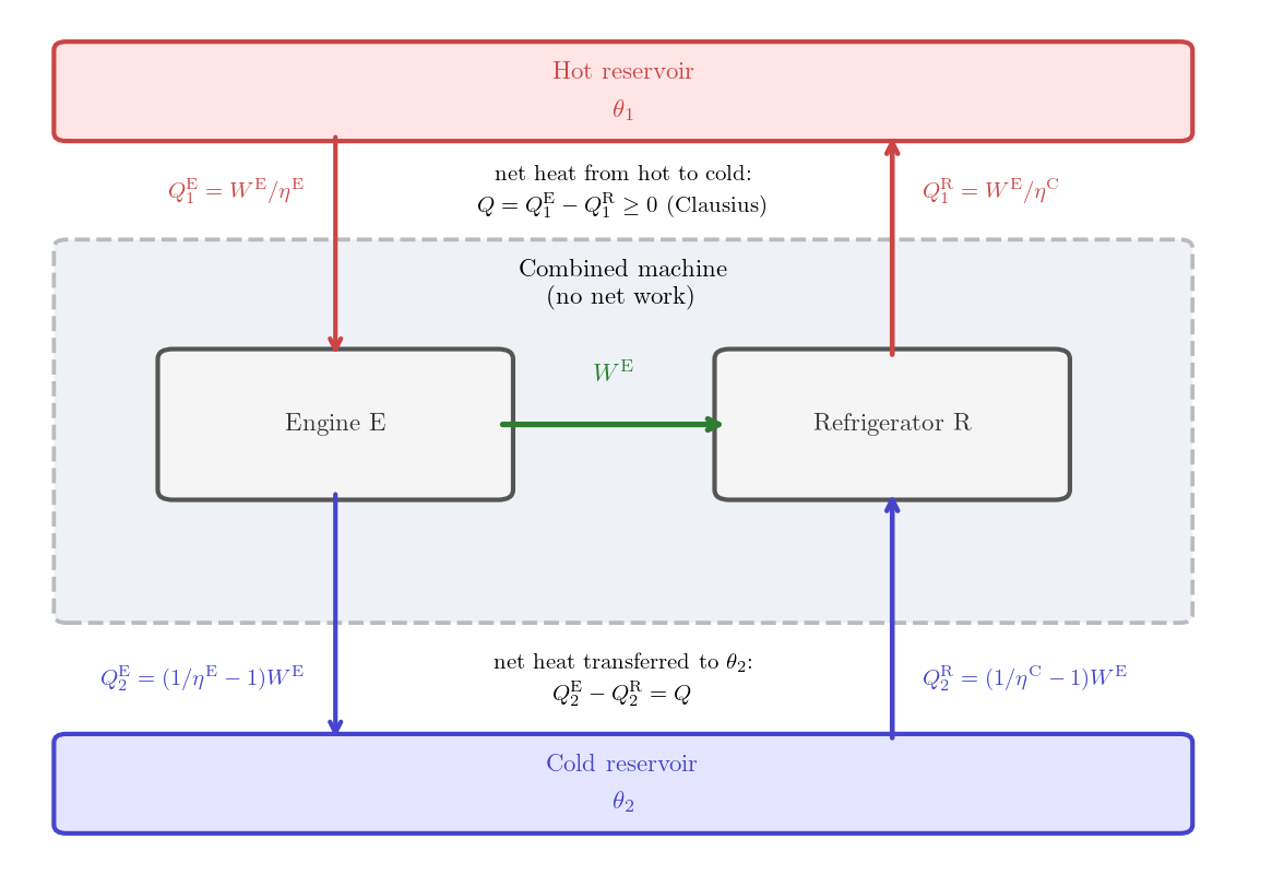
Construction. Since the engine C is reversible, it can be rescaled by a factor \(\lambda = W^{\rm E}/W^{\rm C} > 0\) as described in Section 6.1.1 and run backwards as a refrigerator, which we will call R. In one cycle, this refrigerator absorbs heat \[ Q^{\rm R}_2 = \lambda Q^{\rm C}_2 > 0 \] from the cold reservoir, releases heat \[ Q^{\rm R}_1 = \lambda Q^{\rm C}_1 = \frac{W^{\rm E}}{W^{\rm C}} \frac{W^{\rm C}}{\eta^{\rm C}} = \frac{W^{\rm E}}{\eta^{\rm C}} > 0 \] to the hot reservoir and extracts work \[ W^{\rm R} = \lambda W^{\rm C} = \frac{W^{\rm E}}{W^{\rm C}} W^{\rm C}= W^{\rm E} > 0 \] from the surroundings. Now, run the engine E for one cycle, producing work output \(W^{\rm E}\) and use this work to power the refrigerator R for one cycle. The combined machine consists of the engine E and the refrigerator R running simultaneously, sharing the same two reservoirs. It is clearly cyclic.
Net effect. The engine’s entire work output \(W^{\rm E}\) drives the refrigerator, so the combined machine performs no net work on the surroundings. The net heat transferred by the machine from the hot source to the cold one is \[ Q = Q^{\rm E}_1 - Q^{\rm R}_1 = \left( \frac{1}{\eta^{\rm E}} - \frac{1}{\eta^{\rm C}} \right) W^{\rm E} . \]
Conclusions. Clausius’s statement (Principle 5.1) implies \(Q \ge 0\). Since E is a heat engine, the work produced by E is strictly positive, i.e. \(W^{\rm E} > 0\). Then \(Q \ge 0\) is equivalent to \(\frac{1}{\eta^{\rm E}} - \frac{1}{\eta^{\rm C}} \ge 0\). Both \(\eta^{\rm E}\) and \(\eta^{\rm C}\) are strictly positive (each engine produces positive work from positive heat input), so inverting reciprocals preserves the direction of the inequality and gives \(\eta^{\rm C} \ge \eta^{\rm E}\), which is the desired efficiency bound \(\eta^{\rm E} \le \eta^{\rm C}\).
6.1.3 Proof of Carnot’s theorem, part two
We want to prove the first statement of Theorem 6.1, i.e. all reversible engines that work between the same pair of reservoirs have the same efficiency. This is easily proved by using the efficiency bound proved in Section 6.1.2 twice. Name C’ and C’’ the two reversible engines. Since C’ is reversible and C’’ is generic, we get the efficiency bound \(\eta^{\rm C''} \le \eta^{\rm C'}\). Since C’’ is reversible and C’ is generic, we get the efficiency bound \(\eta^{\rm C'} \le \eta^{\rm C''}\). The two simultaneous inequalities imply the equality \(\eta^{\rm C'} = \eta^{\rm C''}\).
6.2 Definition of absolute temperature
Given a reversible engine C which absorbs heat \(Q^{\rm C}_1\) from a hot reservoir at temperature \(\theta_1\) and releases heat \(Q^{\rm C}_2\) to a cold reservoir at temperature \(\theta_2\), Carnot’s theorem implies that its efficiency \(\eta^{\rm C} = 1 - Q^{\rm C}_2/Q^{\rm C}_1\) and, therefore, the ratio \(Q^{\rm C}_2/Q^{\rm C}_1\) are functions of \(\theta_1\) and \(\theta_2\) only and they do not depend on the details of the engine, i.e. \[ \frac{Q^{\rm C}_2}{Q^{\rm C}_1} = f(\theta_2,\theta_1). \tag{6.1}\] Notice that, by construction, at this stage the function \(f(\theta_2,\theta_1)\) makes sense only if \(\theta_2 < \theta_1\).
Consider now a third reservoir with temperature \(\theta_3\) such that \(\theta_1 > \theta_2 > \theta_3\), and consider a second reversible engine C’ which works between \(\theta_2\) and \(\theta_3\). The engine \(C'\) is rescaled in such a way that, in one cycle, it absorbs from the reservoir at \(\theta_2\) exactly the same amount of heat released by C, i.e. \(Q^{\rm C'}_2 = Q^{\rm C}_2 > 0\). We denote by \(Q^{\rm C'}_3\) the heat released by C’ to the reservoir at \(\theta_3\). Then, Equation 6.1 applied to C’ reads \[ \frac{Q^{\rm C'}_3}{Q^{\rm C'}_2} = f(\theta_3,\theta_2). \tag{6.2}\]
We define a combined machine consisting of the two engines C and C’ running simultaneously, sharing the same reservoir at \(\theta_2\) and working between \(\theta_1\) and \(\theta_3\). The combined machine is cyclic, absorbs heat \(Q^{\rm C}_1>0\) from the hot reservoir at \(\theta_1\), releases heat \(Q^{\rm C'}_3>0\) to the cold reservoir at \(\theta_3\). It does not exchange net heat with the reservoir at \(\theta_2\) by construction and it produces net work given by the sum of the works produced by the individual engines. Therefore, the combined machine is a reversible engine itself. Equation 6.1 applied to the combined machine reads \[ \frac{Q^{\rm C'}_3}{Q^{\rm C}_1} = f(\theta_3,\theta_1). \tag{6.3}\] Now, combining the above three equations with the condition that no net heat is exchanged with the reservoir at \(\theta_2\) (i.e. \(Q^{\rm C}_2 = Q^{\rm C'}_2\)), we get \[ f(\theta_3,\theta_1) = \frac{Q^{\rm C'}_3}{Q^{\rm C}_1} = \frac{Q^{\rm C'}_3}{Q^{\rm C'}_2} \frac{Q^{\rm C}_2}{Q^{\rm C}_1} = f(\theta_3,\theta_2) f(\theta_2,\theta_1). \tag{6.4}\] At this stage, the above equation makes sense only if \(\theta_1 > \theta_2 > \theta_3\).
Equation 6.4 motivates extending \(f\) to all temperature pairs. In what follows, the symbols \(\theta_1\) and \(\theta_2\) are reused as generic labels for the two arguments of \(f\), no longer tied to the hot/cold roles they played in the construction above. The original definition (Equation 6.1) was given for the case where the first slot holds the colder temperature, so it remains in force whenever \(\theta_1 < \theta_2\). For the remaining cases we set \[ f(\theta_1, \theta_2) = \begin{cases} 1 & \text{if } \theta_1 = \theta_2 \\ 1/f(\theta_2, \theta_1) & \text{if } \theta_1 > \theta_2 \end{cases} \ . \] With this extended definition, one easily checks that the composition rule \[ f(\theta_3,\theta_1) = f(\theta_3,\theta_2) f(\theta_2,\theta_1) \tag{6.5}\] holds for all temperatures \(\theta_1\), \(\theta_2\) and \(\theta_3\).
The absolute temperature scale is defined as follows. One chooses a reference state, which is customarily taken to be the triple point of water, with empirical temperature \(\theta_{\rm tr}\). The absolute temperature \(T^{\rm abs}\) of a state with empirical temperature \(\theta\) is defined by \[ T^{\rm abs} = f(\theta, \theta_{\rm tr}) \times 273.16\ \mathrm{K} \ . \] Since \(f(\theta_{\rm tr}, \theta_{\rm tr}) = 1\), the triple point of water has absolute temperature \(T^{\rm abs}_{\rm tr} = 273.16\ \mathrm{K}\) by construction. The composition rule (Equation 6.5) implies that the heat ratio for a reversible engine can be expressed in terms of absolute temperatures as \[ \frac{Q^{\rm C}_2}{Q^{\rm C}_1} = f(\theta_2,\theta_1) = \frac{f(\theta_2, \theta_{\rm tr})}{f(\theta_1, \theta_{\rm tr})} = \frac{T^{\rm abs}_2}{T^{\rm abs}_1}. \] Therefore, the efficiency of a reversible engine can be expressed in terms of absolute temperatures as \[ \eta^{\rm C} = 1 - \frac{Q^{\rm C}_2}{Q^{\rm C}_1} = 1 - \frac{T^{\rm abs}_2}{T^{\rm abs}_1}. \]
Absolute temperature \(T\) — defined via the Carnot heat ratio: \(Q_2/Q_1 = T_2/T_1\) for any reversible engine. Universal; independent of working substance. Fixed by assigning \(273.16\ \mathrm{K}\) to the triple point of water.
6.2.1 Relation to the ideal-gas temperature
The Carnot engine constructed in the previous lecture (Chapter 5) uses an ideal gas as working substance and operates between reservoirs at ideal-gas temperatures \(T_1\) and \(T_2\). Its efficiency was computed in Equation 5.8: \[ \eta^{\rm C} = 1 - \frac{T_2}{T_1}. \] Comparing with the expression above, the absolute temperature \(T^{\rm abs}\) and the ideal-gas temperature \(T\) agree on the ratio \(T^{\rm abs}_2/T^{\rm abs}_1 = T_2/T_1\) for any pair of states accessible to an ideal gas. Since both scales are fixed by the same reference point (the triple point of water at \(273.16\ \mathrm{K}\)), the two temperatures are not merely proportional: they are identical, \[ T^{\rm abs} = T. \]
The absolute temperature scale is, however, more general than the ideal-gas scale. The ideal-gas temperature is measured by bringing a dilute gas thermometer into thermal equilibrium with the system of interest; it is therefore defined only in temperature ranges where a real gas can be made to behave ideally. At very low temperatures all gases liquefy, and at very high temperatures all gases ionize, before the ideal-gas limit is reached; in both regimes the ideal-gas thermometer ceases to be operational. The absolute temperature, by contrast, is defined via the efficiency of any reversible engine, regardless of the working substance, and is therefore well defined at all temperatures. The two scales agree wherever the ideal-gas thermometer is applicable, so no experimental result is changed; but the absolute scale extends the concept of temperature beyond the reach of any gas thermometer.
From this point on we write \(T\) for the absolute temperature and drop the superscript \({}^{\rm abs}\).
6.3 Clausius inequalities
There are two versions of Clausius inequality. The first one applies to generic cyclic machines. The second one applies to quasi-static cyclic processes. The second inequality follows from the first one and leads to the definition of entropy.
T 6.2 (First Clausius inequality) A generic cyclic machine (Figure 5.2) which, in one cycle, absorbs heat \(Q_i\) from \(n\) reservoirs at (absolute) temperatures \(T_1, T_2, \ldots, T_n\) and delivers \(W\) to the surroundings, satisfies \[ \sum_{i=1}^n \frac{Q_i}{T_i} \leq 0. \tag{6.6}\] If the machine is reversible, the equality holds, i.e. \(\sum_{i=1}^n \frac{Q_i}{T_i} = 0\).
The second Clausius inequality involves the integral of \(\delta Q / T\) along a quasi-static process. This is a line integral defined in the same manner as you have seen in Mechanics for the work done by a force along a path and Electromagnetism for the circulation of a magnetic field along a loop. Let us see how to define this line integral in the context of thermodynamics.
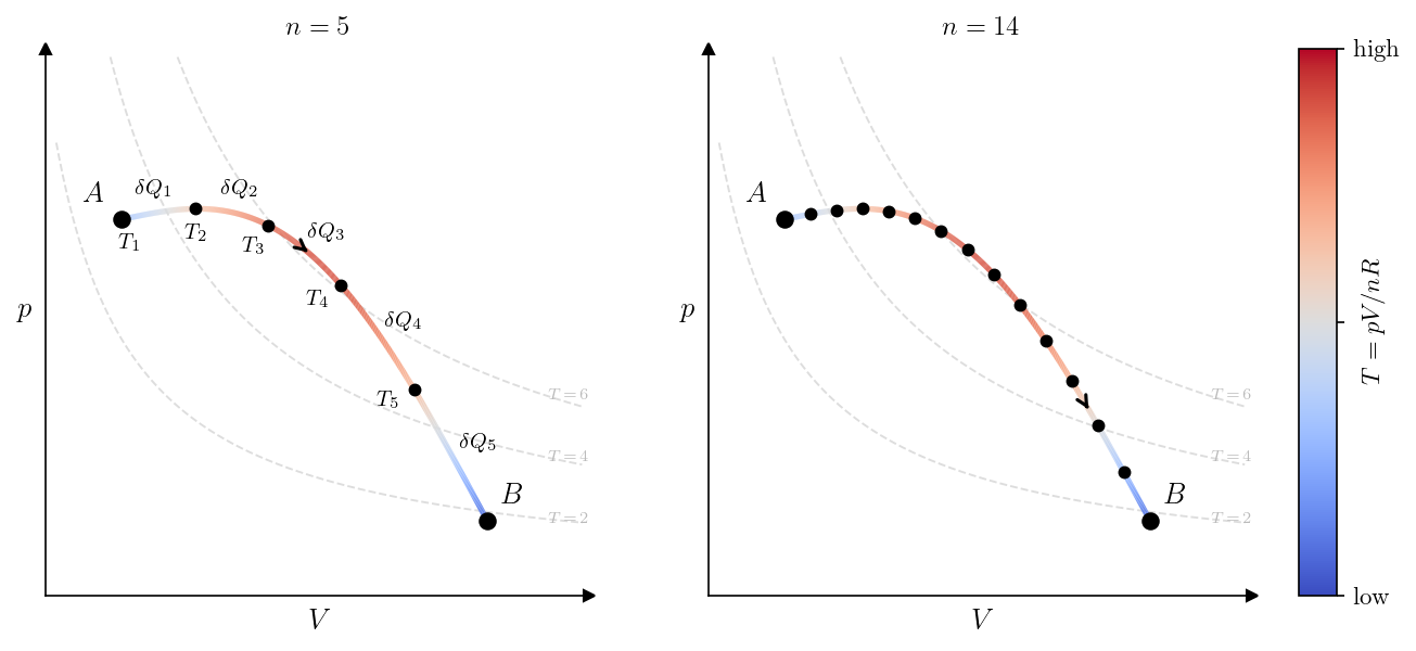
A quasi-static process consists of a continuous succession of equilibrium states. The process traces a curve \(\gamma\) in the space of equilibrium states. The temperature \(T\) is a state function, so it has a well-defined value at every point of \(\gamma\). For instance, for a gas or liquid, a quasi-static process can be represented as a curve in the \((V, p)\) plane and the temperature at each point of the curve is given by the equation of state as shown in Figure 6.2.
Consider such a quasi-static process taking the system from state \(A\) to state \(B\). Subdivide \(\gamma\) into \(n\) small steps by choosing intermediate states along the curve. In the \(k\)-th step, the system starts at temperature \(T_k\) and absorbs a small heat \(\delta Q_k\). The Riemann sum \[ \sum_{k=1}^{n} \frac{\delta Q_k}{T_k} \] approximates the cumulative ratio of heat to temperature along the process. The line integral is defined as the limit of this sum as the subdivision is refined: \[ \int_{\gamma} \frac{\delta Q}{T} = \lim_{n \to \infty} \sum_{k=1}^{n} \frac{\delta Q_k}{T_k}. \]
Line integral \(\int_\gamma \delta Q/T\) — limit of the Riemann sum \(\sum_k \delta Q_k/T_k\) as the subdivision of the path \(\gamma\) is refined. Path-dependent in general; path-independent for reversible processes.
In terms of a parametrization, let \(s \mapsto (V(s), p(s))\) be any parametrization of \(\gamma\) by \(s \in [s_A, s_B]\), with \(s_A\) and \(s_B\) corresponding to \(A\) and \(B\). Then \[ \int_{\gamma} \frac{\delta Q}{T} = \int_{s_A}^{s_B} \frac{\dot{Q}(s)}{T(s)} \, \mathrm{d}s, \] where \(T(s)\) is the temperature of the system at \(s\) and \(Q(s)\) is the heat absorbed by the system from the beginning of the process until \(s\). Notice that \(\delta Q = \dot{Q}(s) \mathrm{d}s\) is the heat absorbed during the infinitesimal step from \(s\) to \(s + \mathrm{d}s\). We notice that, in general, the value of the integral depends on the path \(\gamma\), not only on the endpoints. When \(\gamma\) is a closed curve, the integral is written \(\oint_{\gamma} \delta Q / T\). We are now ready to state the second Clausius inequality.
T 6.3 (Second Clausius inequality) For any generic quasi-static cyclic process, represented by the closed curve \(\gamma\) in the space of equilibrium states, the following inequality holds: \[ \oint_{\gamma} \frac{\delta Q}{T} \leq 0. \tag{6.7}\] If the quasi-static cyclic process is reversible, the equality holds, i.e. \(\oint_{\gamma} \frac{\delta Q}{T} = 0\).
There is an essential difference in the meaning of the symbol \(T\) between the two inequalities. In the first inequality, \(T_i\) is the temperature of the \(i\)-th reservoir and not of the machine. In fact, the machine is not even assumed to be in equilibrium during the cycle and its temperature is not defined at all times. In the second inequality, \(T\) is the temperature of the system along the process and the system is assumed to be in equilibrium at all times.
6.3.1 Proof of the first Clausius inequality
Consider a cyclic machine M which, in one cycle, absorbs heat \(Q_i\) from reservoir \(i\) at temperature \(T_i\) (\(i = 1, \ldots, n\)) and delivers work \(W = \sum_i Q_i\) to the surroundings.
Construction. Choose a reference temperature \(T_0 < T_i\) for all \(i\). For each reservoir \(i\), introduce a Carnot engine \(C_i\) operating between \(T_0\) and \(T_i\), rescaled so that it exchanges exactly \(Q_i\) with reservoir \(i\) per cycle. By the Carnot heat ratio (Equation 6.1 and the definition of absolute temperature in Section 6.2), the heat exchanged by \(C_i\) with the cold reservoir at \(T_0\) is \[ Q_{0,i} = \frac{T_0}{T_i}\, Q_i. \] If \(Q_i > 0\), machine M absorbs heat from reservoir \(i\); engine \(C_i\) runs as a refrigerator, consuming work to deposit \(Q_i\) back into reservoir \(i\), with net exchange zero. If \(Q_i < 0\), machine M releases heat to reservoir \(i\); engine \(C_i\) runs as a heat engine, extracting \(|Q_i|\) from reservoir \(i\) and depositing heat into \(T_0\), again leaving reservoir \(i\) with zero net exchange. The combined machine M \(+ \{C_i\}_{i=1}^n\) is therefore cyclic and exchanges heat only with the single reservoir at \(T_0\).
Net effect. The total heat absorbed from \(T_0\) by the combined machine in one cycle is \[ Q_0 = \sum_{i=1}^n Q_{0,i} = T_0 \sum_{i=1}^n \frac{Q_i}{T_i}. \] Since the combined machine is cyclic and exchanges heat with no reservoir other than \(T_0\), energy conservation implies that the total work it delivers to the surroundings equals \(Q_0\).
Conclusions. The combined machine is cyclic and interacts with only one reservoir at \(T_0\). Kelvin’s statement (Consequence 5.1) implies that it cannot deliver positive work, i.e. \(Q_0 \leq 0\). Since \(T_0 > 0\), \[ \sum_{i=1}^n \frac{Q_i}{T_i} \leq 0. \] If M is reversible, the same argument applied to M running in reverse (for which the heat exchanged with each reservoir changes sign) gives \(\sum_i Q_i/T_i \geq 0\). The two inequalities together imply \(\sum_i Q_i/T_i = 0\).
6.3.2 Proof of the second Clausius inequality
The second inequality follows directly from the first by approximating the quasi-static process by a sequence of discrete steps and taking the limit as the number of steps goes to infinity.
A quasi-static cyclic process is represented by a closed curve \(\gamma\) in the space of equilibrium states. Subdivide \(\gamma\) into \(n\) steps. In the \(k\)-th step the system passes through a range of equilibrium states, but as \(n\) grows the steps shrink and the temperature variation within each step becomes arbitrarily small. For large enough \(n\), the temperature within the \(k\)-th step is therefore essentially constant and equal to some representative value \(T_k\). Furthermore, because the process is quasi-static, the temperature difference between the system and its surroundings is infinitesimal at every instant; the surroundings therefore act, to within an infinitesimal correction, as a reservoir at the same temperature \(T_k\) as the system. Treating each step as an exchange of heat \(\delta Q_k\) with a reservoir at temperature \(T_k\), the \(n\)-step cyclic process falls within the scope of the first Clausius inequality (Theorem 6.2): \[ \sum_{k=1}^{n} \frac{\delta Q_k}{T_k} \leq 0. \] Taking the limit \(n \to \infty\) as the subdivision is refined, the left-hand side converges to the line integral \(\oint_\gamma \delta Q/T\) by definition above, giving \[ \oint_{\gamma} \frac{\delta Q}{T} \leq 0. \] If the quasi-static cyclic process is reversible, reversing it changes the sign of every \(\delta Q_k\) (since the system traverses the same states in the opposite order, exchanging the same amounts of heat with opposite sign), while the temperatures \(T_k\) are unchanged. The same argument applied to the reversed process gives \(\oint_\gamma \delta Q/T \geq 0\), and together with the inequality above this implies \(\oint_\gamma \delta Q/T = 0\).
6.4 Definition of entropy
The second Clausius inequality for reversible processes has a remarkable consequence: the line integral \(\int_\gamma \delta Q / T\) along a reversible quasi-static path depends only on the endpoints, not on the path.
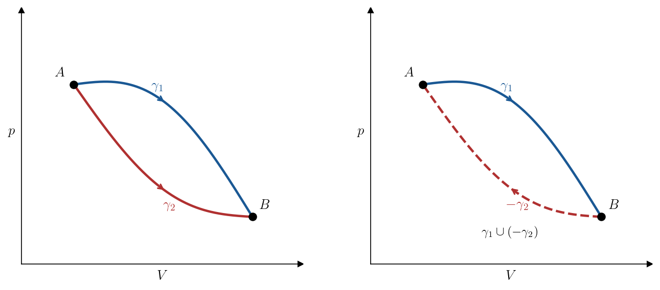
To see this, let \(\gamma_1\) and \(\gamma_2\) be any two reversible quasi-static paths from state \(A\) to state \(B\) (Figure 6.3, left). Denote by \(-\gamma_2\) the same path traversed in reverse, from \(B\) to \(A\). The concatenation \(\gamma_1 \cup (-\gamma_2)\) is a closed reversible quasi-static curve (Figure 6.3, right), so the second Clausius inequality (Theorem 6.3) gives \[ 0 = \oint_{\gamma_1 \cup (-\gamma_2)} \frac{\delta Q}{T} = \int_{\gamma_1} \frac{\delta Q}{T} - \int_{\gamma_2} \frac{\delta Q}{T}. \] Therefore \(\int_{\gamma_1} \delta Q/T = \int_{\gamma_2} \delta Q/T\): the integral is the same for every reversible path from \(A\) to \(B\).
This means that, for reversible quasi-static processes, \(\int_\gamma \delta Q/T\) is a function of the endpoints alone. We can therefore define a state function as follows.
Definition 6.1 (Entropy) Fix a reference equilibrium state \(O\). The entropy \(S\) of an equilibrium state \(A\) is defined by \[ S(A) = S(O) + \int_{\gamma_{OA}} \frac{\delta Q}{T}, \tag{6.8}\] where \(\gamma_{OA}\) is any reversible quasi-static path from \(O\) to \(A\), and \(S(O)\) is an arbitrary constant.
Entropy \(S\) — a state function defined by \(S(A) = S(O) + \int_{\gamma_{OA}} \delta Q/T\) along any reversible quasi-static path from reference state \(O\) to \(A\). Units: J K\(^{-1}\); extensive.
The definition is well-posed because the integral is path-independent. The entropy difference between two states \(A\) and \(B\) is therefore \[ S(B) - S(A) = \int_{\gamma_{AB}} \frac{\delta Q}{T}, \tag{6.9}\] where \(\gamma_{AB}\) is any reversible quasi-static path from \(A\) to \(B\).
A few remarks are in order.
Entropy is measurable. The definition Equation 6.9 is operational: to measure the entropy difference between two states \(A\) and \(B\), one designs any reversible quasi-static process connecting them, measures the heat \(\delta Q\) exchanged at each stage and the temperature \(T\) at which it is exchanged, and evaluates the integral. This is not merely a theoretical construction: calorimetric measurements of \(\delta Q / T\) along controlled processes are how entropy differences are determined in the laboratory. Entropy is no more abstract than internal energy: both are defined by integrals of measurable quantities along controlled processes.
Entropy is a state function. Like internal energy \(U\), temperature \(T\), or pressure \(p\), entropy \(S\) is a property of an equilibrium state, not of a process. It is defined up to an additive constant, just as potential energy is. The reference value \(S(O)\) will be fixed later in the course.
Units. From the definition, \([S] = [Q]/[T] = \text{J}/\text{K}\).
Entropy is extensive. If a system is the union of two independent subsystems with entropies \(S_1\) and \(S_2\), the total entropy is \(S = S_1 + S_2\). This follows because heat and temperature are extensive and intensive, respectively, and the integral is additive over subsystems.
6.5 Problems
Problem 6.1 A reversible cyclic engine (working substance unspecified) operates between two reservoirs at absolute temperatures \(T_1 = 600\ \mathrm{K}\) and \(T_2 = 350\ \mathrm{K}\). Per cycle it absorbs \(Q_1 = 800\ \mathrm{J}\) from the hot reservoir. (In this problem and the next, \(Q_1\) and \(Q_2\) are positive magnitudes, in the heat-engine/heat-pump convention of lecture 5.)
Compute the efficiency \(\eta^{\rm C}\) using Equation 5.8 and the heat \(Q_2\) released to the cold reservoir.
Compute the work \(W\) delivered to the surroundings.
The efficiency depends only on \(T_1\) and \(T_2\), not on the working substance. Explain in one sentence why this universality follows from Carnot’s theorem (Theorem 6.1), independent of any particular construction such as the ideal-gas Carnot cycle that produced Equation 5.8.
Problem 6.2 A reversible Carnot heat pump operates between absolute temperatures \(T_1 = 320\ \mathrm{K}\) (interior) and \(T_2 = 280\ \mathrm{K}\) (exterior). Per cycle it delivers \(Q_1 = 5.0\ \mathrm{kJ}\) to the interior. Recall the COP definitions of Equation 5.9 and Equation 5.10.
Express \(\mathrm{COP}_{\rm HP}\) as a function of \(T_1\) and \(T_2\) alone, and evaluate it numerically.
Compute the work \(W\) consumed per cycle and the heat \(Q_2\) extracted from the exterior.
Verify the identity \(\mathrm{COP}_{\rm HP} = \mathrm{COP}_{\rm R} + 1\) from the absolute-temperature expressions of both COPs.
Problem 6.3 A cyclic machine exchanges heat with two reservoirs at absolute temperatures \(T_1 = 500\ \mathrm{K}\) (hot) and \(T_2 = 300\ \mathrm{K}\) (cold), with the generic sign convention of Figure 5.2 (\(Q_i\) positive if absorbed by the machine from reservoir \(i\)). For each case below, (i) compute \(\sum_i Q_i/T_i\) and use the first Clausius inequality (Theorem 6.2) to classify the machine as physically impossible, irreversible, or reversible; (ii) compute \(W = Q_1 + Q_2\) and identify whether the machine is a heat engine, refrigerator, dissipator, or none of the above.
\(Q_1 = +1500\ \mathrm{J}\), \(Q_2 = -900\ \mathrm{J}\).
\(Q_1 = +1500\ \mathrm{J}\), \(Q_2 = -1050\ \mathrm{J}\).
\(Q_1 = +1500\ \mathrm{J}\), \(Q_2 = -800\ \mathrm{J}\).
\(Q_1 = -300\ \mathrm{J}\), \(Q_2 = +800\ \mathrm{J}\).
Problem 6.4 Like Problem 6.3, with \(T_1 = 400\ \mathrm{K}\), \(T_2 = 250\ \mathrm{K}\), and:
\(Q_1 = +800\ \mathrm{J}\), \(Q_2 = -500\ \mathrm{J}\).
\(Q_1 = +800\ \mathrm{J}\), \(Q_2 = -600\ \mathrm{J}\).
\(Q_1 = +800\ \mathrm{J}\), \(Q_2 = -400\ \mathrm{J}\).
\(Q_1 = 0\), \(Q_2 = -500\ \mathrm{J}\).
Problem 6.5 A monatomic ideal gas (\(c_V = 3R/2\)) with \(n = 1.0\ \mathrm{mol}\), initially at \(T_A = 300\ \mathrm{K}\) and \(V_A = 10.0\ \mathrm{L}\), is taken reversibly through the following two-step path to state B:
- Leg A \(\to\) C: isothermal expansion at \(T_A\) from \(V_A\) to \(V_C = 20.0\ \mathrm{L}\).
- Leg C \(\to\) B: isochoric heating at \(V_C\) from \(T_A\) to \(T_B = 450\ \mathrm{K}\).
On each leg, compute the heat \(\delta Q\) exchanged by the gas and the entropy change \(\Delta S = \int \delta Q/T\) of the gas, using the definition Equation 6.9.
Compute the total entropy change \(S(B) - S(A)\).
Verify that the result is consistent with the general formula \(\Delta S = nc_V\ln(T_B/T_A) + nR\ln(V_B/V_A)\) derived in Problem 6.13.
Problem 6.6 A diatomic ideal gas in the rotational plateau (\(c_V = 5R/2\), \(c_p = 7R/2\)) with \(n = 0.50\ \mathrm{mol}\), initially at \(T_A = 400\ \mathrm{K}\) and \(V_A = 5.0\ \mathrm{L}\), is taken reversibly through the following two-step path to state B:
- Leg A \(\to\) C: isobaric expansion at \(p_A\) from \(T_A\) to \(T_C = 500\ \mathrm{K}\).
- Leg C \(\to\) B: isothermal expansion at \(T_C\) from \(V_C\) to \(V_B = 12.0\ \mathrm{L}\).
Determine \(p_A\) and \(V_C\).
On each leg, compute \(\delta Q\) exchanged by the gas and the entropy change \(\Delta S\).
Compute the total entropy change \(S(B) - S(A)\).
Problem 6.7 A reversible cyclic machine exchanges heat with three reservoirs at absolute temperatures \(T_1 = 600\ \mathrm{K}\), \(T_2 = 400\ \mathrm{K}\), \(T_3 = 300\ \mathrm{K}\), with the generic sign convention of Figure 5.2. In one cycle the machine absorbs \(Q_1 = +900\ \mathrm{J}\) from reservoir 1 and exchanges \(Q_2 = -200\ \mathrm{J}\) with reservoir 2.
Use the equality case of the first Clausius inequality (Theorem 6.2) to determine \(Q_3\).
Compute the net work \(W\) delivered to the surroundings.
Compute the efficiency \(\eta = W/Q_{\rm in}\), where \(Q_{\rm in}\) is the sum of the heats absorbed (i.e. only the \(Q_i > 0\) terms).
Verify that \(\eta < 1 - T_3/T_1\), the Carnot bound for an engine working between the hottest and coldest reservoirs only. The inequality is strict because this machine also exchanges heat with the intermediate reservoir \(T_2\) (the general bound is established in Problem 6.12).
Problem 6.8 Like Problem 6.7, with three reservoirs at \(T_1 = 500\ \mathrm{K}\), \(T_2 = 350\ \mathrm{K}\), \(T_3 = 250\ \mathrm{K}\). Per cycle the machine absorbs \(Q_1 = +1000\ \mathrm{J}\) from reservoir 1 and releases \(Q_3 = -700\ \mathrm{J}\) to reservoir 3. The machine is reversible.
Use the equality case of the first Clausius inequality (Theorem 6.2) to determine \(Q_2\), and identify whether reservoir 2 absorbs or releases heat.
Compute the work \(W\) delivered to the surroundings.
Compute the efficiency \(\eta = W/Q_{\rm in}\), with \(Q_{\rm in}\) defined as in Problem 6.7 (sum of the positive \(Q_i\) only), and compare with \(1 - T_3/T_1\).
Problem 6.9 (More demanding. Mirrors Problem 5.13 for refrigerators.) A hypothetical refrigerator \(X\) operates between reservoirs at absolute temperatures \(T_1 > T_2\). Per cycle it extracts \(Q_2^X > 0\) from the cold reservoir, consumes work \(W^X > 0\) from the surroundings, and deposits \(Q_1^X = W^X + Q_2^X\) into the hot reservoir. Assume its coefficient of performance exceeds the Carnot value: \[ \mathrm{COP}_{\rm R}^X = \frac{Q_2^X}{W^X} > \frac{T_2}{T_1 - T_2} = \mathrm{COP}_{\rm R}^{\rm C}. \] Combine \(X\) with a reversible Carnot heat engine operating between the same two reservoirs, scaled so the engine delivers exactly the work \(W^X\) per combined cycle, which is supplied to \(X\).
Express, in terms of \(W^X\), \(T_1\), \(T_2\), the heat \(Q_1^{\rm C}\) absorbed by the Carnot engine from the hot reservoir and the heat \(Q_2^{\rm C}\) released to the cold reservoir per combined cycle.
Compute the net heat \(\Delta Q_1\) exchanged with the hot reservoir and the net heat \(\Delta Q_2\) exchanged with the cold reservoir, per combined cycle, and show that \(\Delta Q_1 < 0\) and \(\Delta Q_2 > 0\).
Show that the combined cyclic machine transfers heat from the cold reservoir to the hot reservoir without exchanging net work with the surroundings, in violation of Clausius’s statement (Principle 5.1).
Conclude that every refrigerator operating between two reservoirs at \(T_1\) and \(T_2\) satisfies \(\mathrm{COP}_{\rm R} \le T_2/(T_1 - T_2)\).
Problem 6.10 (More demanding.) Repeat the argument of Problem 6.9 for a hypothetical heat pump \(X\) with \(\mathrm{COP}_{\rm HP}^X > T_1/(T_1 - T_2)\). Show that combining \(X\) with a Carnot engine produces a Clausius-violating combined machine, and conclude that every heat pump satisfies \[ \mathrm{COP}_{\rm HP} \le \frac{T_1}{T_1 - T_2}. \]
Problem 6.11 (More demanding.) A cyclic engine operates between three reservoirs at absolute temperatures \(T_1 > T_2 > T_3\). In one cycle it absorbs \(Q_1 > 0\) from reservoir 1 and \(Q_2 > 0\) from reservoir 2, and releases \(Q_3 > 0\) to reservoir 3 (the symbols \(Q_1, Q_2, Q_3\) are positive magnitudes). The work delivered to the surroundings is \(W = Q_1 + Q_2 - Q_3 > 0\). Define the efficiency as \(\eta = W/Q_{\rm in}\) where \(Q_{\rm in} = Q_1 + Q_2\).
Apply the first Clausius inequality (Theorem 6.2) to this machine. Recall that the inequality is stated for signed heats (positive if absorbed by the machine), so when expressing it in terms of the positive magnitudes above, the released \(Q_3\) enters with a minus sign.
Eliminate \(Q_3\) via the First Law and show that \[ \eta \le 1 - \frac{T_3}{Q_{\rm in}}\left(\frac{Q_1}{T_1} + \frac{Q_2}{T_2}\right). \]
Let \(\lambda = Q_1/Q_{\rm in} \in [0,1]\). Show that the right-hand side of part (b) can be rewritten as a convex combination of pairwise Carnot efficiencies: \[ \eta \le \lambda\,\eta^{\rm C}_{13} + (1-\lambda)\,\eta^{\rm C}_{23}, \qquad \eta^{\rm C}_{ij} := 1 - \frac{T_j}{T_i}. \]
Conclude that \(\eta \le \eta^{\rm C}_{13}\) (the Carnot bound between the hottest and coldest reservoirs is the most favourable). Show that the bound is approached in the limit \(\lambda \to 1\) (i.e. \(Q_2 \to 0\), the machine becoming effectively a two-reservoir engine between \(T_1\) and \(T_3\)) with reversible operation.
Problem 6.12 (More demanding.) A cyclic engine operates between three reservoirs at absolute temperatures \(T_1 > T_2 > T_3\). In one cycle it absorbs \(Q_1 > 0\) from reservoir 1 and releases \(Q_2 > 0\) to reservoir 2 and \(Q_3 > 0\) to reservoir 3 (positive magnitudes). Define the efficiency \(\eta = W/Q_1\) with \(W = Q_1 - Q_2 - Q_3 > 0\), and let \(\mu = Q_2/(Q_2 + Q_3) \in [0,1]\) be the fraction of waste heat dumped at the warmer cold reservoir.
Apply the first Clausius inequality (signed-heats convention) and show that the constraint can be written as \[ \frac{Q_2}{T_2} + \frac{Q_3}{T_3} \ge \frac{Q_1}{T_1}. \]
Parametrising the waste heats by \(\mu\) as above, show that \[ \eta \le 1 - \frac{T_2 T_3}{T_1\,[\mu T_3 + (1-\mu)\,T_2]}. \]
Verify that at \(\mu = 0\) (all waste heat dumped at the coldest reservoir) the bound reduces to \(\eta^{\rm C}_{13} = 1 - T_3/T_1\), and at \(\mu = 1\) (all waste heat dumped at the warmer cold reservoir) it reduces to \(\eta^{\rm C}_{12} = 1 - T_2/T_1\).
Show that the bound is monotonically decreasing in \(\mu\), so it is maximised at \(\mu = 0\). Conclude that for any split of waste heat, \(\eta \le \eta^{\rm C}_{13}\), the same bound as in Problem 6.11.
Problem 6.13 (Forward-looking: previews the first \(T\,dS\) equation, Lecture 7.) An ideal gas with \(n\) moles and constant molar heat capacity \(c_V\) is in equilibrium at state A \((T_1, V_1)\) and at state B \((T_2, V_2)\). We compute the entropy difference \(S(B) - S(A)\) using two different reversible quasi-static paths from A to B, and verify they agree.
Path I: isochoric heating at \(V_1\) from \(T_1\) to \(T_2\), then isothermal expansion at \(T_2\) from \(V_1\) to \(V_2\). Compute \(\delta Q\) and \(\Delta S\) on each leg, and sum.
Path II: isothermal expansion at \(T_1\) from \(V_1\) to \(V_2\), then isochoric heating at \(V_2\) from \(T_1\) to \(T_2\). Compute \(\delta Q\) and \(\Delta S\) on each leg, and sum.
Verify that both paths give \[ S(B) - S(A) = n c_V \ln\frac{T_2}{T_1} + nR \ln\frac{V_2}{V_1}. \]
In Lecture 7, this formula will be re-derived in one step using the first \(T\,dS\) equation \(T\,dS = nc_V\,dT + (nRT/V)\,dV\), which is itself a consequence of combining the First Law for a reversible process with the definition of entropy.
Problem 6.14 (Forward-looking: the entropy in the variables \((T,p)\).) An ideal gas with \(n\) moles and constant molar heat capacity \(c_p\) is in equilibrium at state A \((T_1, p_1)\) and at state B \((T_2, p_2)\).
Use the reversible two-step path A \(\to\) C \(\to\) B with C \(= (T_2, p_1)\) (isobaric heating at \(p_1\), then isothermal compression/expansion at \(T_2\)) to compute the entropy difference \(S(B) - S(A)\).
Show that \[ S(B) - S(A) = n c_p \ln\frac{T_2}{T_1} - nR \ln\frac{p_2}{p_1}. \]
Verify that this is equivalent to the result of Problem 6.13 by using the ideal-gas equation of state \(pV = nRT\) and the Mayer relation \(c_p - c_V = R\).
This \((T,p)\) form is the second \(T\,dS\) equation, \(T\,dS = nc_p\,dT - (nRT/p)\,dp\); it follows in one step once the enthalpy is introduced, in Lecture 9.
Problem 6.15 (Forward-looking: previews \(\Delta S_{\rm univ} > 0\) for irreversible processes, Lecture 7.) An ideal gas with \(n\) moles, initially in equilibrium at temperature \(T\) and confined to volume \(V_1\), expands freely into a vacuum to occupy the larger volume \(V_2 > V_1\). The container is rigid and thermally insulated (Figure 5.1).
Apply the First Law to argue that the temperature of the gas after the free expansion equals its initial temperature \(T\). (Hint: \(W=0\), \(Q=0\), and the internal energy of an ideal gas depends only on temperature; see lecture 4.)
The free expansion is irreversible, so \(\int \delta Q/T\) along the actual process is not equal to \(\Delta S\). Use the fact that entropy is a state function (Definition 6.1) to compute \(\Delta S_{\rm sys} = S(T, V_2) - S(T, V_1)\) via a reversible quasi-static path connecting the same two equilibrium endpoints. Identify the path and evaluate the integral.
The surroundings exchange no heat and do no work. Argue that \(\Delta S_{\rm surr} = 0\).
Compute \(\Delta S_{\rm univ} = \Delta S_{\rm sys} + \Delta S_{\rm surr}\) and verify that \(\Delta S_{\rm univ} > 0\). For \(V_2 = 2V_1\), evaluate \(\Delta S_{\rm univ}\) numerically for \(n = 1\ \mathrm{mol}\) and compare with the asymptotic value of the Shannon-entropy proxy \(\tilde S = nR\ln 2\) shown in Figure 5.1.
Problem 6.16 (Forward-looking: previews \(\Delta S_{\rm univ} > 0\) for irreversible heat transfer, Lecture 7.) Two finite bodies, each with constant heat capacity \(C\) (at the conditions of the experiment), are placed in thermal contact inside a thermally isolated rigid enclosure. Initially they are in internal equilibrium at temperatures \(T_A\) and \(T_B\) with \(T_A > T_B\). They are left to equilibrate.
Use energy conservation to determine the common final temperature \(T_f\).
Compute the entropy change of each body. (Hint: although the actual thermalisation is irreversible, each body separately passes from a well-defined initial equilibrium state to a well-defined final equilibrium state; its \(\Delta S\) can be computed by integrating \(\delta Q/T = C\,dT/T\) along a reversible path connecting the same two states.)
Compute the total entropy change of the universe, \(\Delta S_{\rm univ}\), and show that \(\Delta S_{\rm univ} \ge 0\), with equality if and only if \(T_A = T_B\).
For \(T_A = 400\ \mathrm{K}\), \(T_B = 300\ \mathrm{K}\), \(C = 100\ \mathrm{J\,K}^{-1}\), evaluate \(T_f\) and \(\Delta S_{\rm univ}\) numerically. Interpret the sign of \(\Delta S_{\rm univ}\) in the light of the lecture’s claim that thermalisation is irreversible.