8 The Chemical Potential and Conditions of Equilibrium
Part III — Potentials and Equilibrium
Last updated: 15-06-2026
8.1 Open systems and the chemical potential
Every system considered so far has been closed: the amount of substance it contains was fixed, and its internal energy could change only through the work done on it and the heat that crossed its boundary. Many of the processes we now wish to describe break this assumption. When two gases meet across a permeable wall, when a liquid evaporates into the space above it, or when a chemical reaction converts one species into another, the amount of substance in a given part of the system changes. To describe such open systems we promote the amount of substance \(n\) to an independent variable, on the same footing as the entropy and the volume.
We therefore regard the internal energy of a one-component system as a function of three variables, \(U = U(S, V, n)\). Its differential acquires a third term, \[ dU = T\, dS - p\, dV + \mu\, dn, \tag{8.1}\] whose first two coefficients are the temperature and pressure of Lecture 7, now taken at fixed \(n\), \[ T = \left(\frac{\partial U}{\partial S}\right)_{V,n}, \qquad p = -\left(\frac{\partial U}{\partial V}\right)_{S,n}, \] and whose third coefficient defines the chemical potential, \[ \mu = \left(\frac{\partial U}{\partial n}\right)_{S,V} . \tag{8.2}\]
This third term is no new postulate; it is demanded by energy conservation. The First Law allows the internal energy to change only by the energy that crosses the system’s boundary. In a closed system that energy arrives in just two forms, as heat, \(T\, dS\), or as work, \(-p\, dV\). Once the boundary is permeable, matter may cross it as well, and matter carries energy with it: the term \(\mu\, dn\) accounts for the energy transported by the matter exchanged. The First Law is unchanged; we have only allowed for a further channel through which energy may flow.
Being a partial derivative, the chemical potential is defined differentially. It is not the energy of a whole mole of substance, for adding a finite amount would alter the temperature, the pressure and every other property of the system along the way; \(\mu\) refers instead to the addition of an infinitesimal amount \(dn\). Its meaning is read directly from Equation 8.1: hold the entropy and volume fixed, so that the terms \(T\, dS\) and \(p\, dV\) both vanish, and admit an infinitesimal quantity of matter \(dn\). The internal energy then changes by \[ dU = \mu\, dn, \] so the chemical potential is the energy the system gains per mole of matter added, at fixed entropy and volume.
Unlike \(S\), \(V\) and \(n\), the chemical potential is intensive. The internal energy, the volume and the amount of substance are extensive, scaling in proportion to the size of the system (the distinction was drawn in Lecture 2), as is the entropy (Lecture 6). If the system is enlarged by a factor \(\lambda\) at fixed composition, \(U\), \(S\), \(V\) and \(n\) are all multiplied by \(\lambda\), whereas \(\mu\), the ratio of the change in \(U\) to the change in \(n\) at fixed \(S\) and \(V\), is unchanged. Like the temperature and the pressure, \(\mu\) therefore takes a single value throughout a system in internal equilibrium.
There is a further parallel with \(T\) and \(p\). The chemical potential is a property of the equilibrium state, not of any process: its defining derivative is evaluated by imagining a virtual addition of matter, yet the value it returns belongs to the state itself, just as \(T = (\partial U/\partial S)_{V,n}\) and \(p = -(\partial U/\partial V)_{S,n}\) do without anything being changed. A chemical potential is therefore defined at every equilibrium state, that of a closed system no less than an open one, exactly as the pressure of a sealed, rigid vessel is well defined although its volume never changes. Open systems are what motivate treating \(n\) as a variable and what give \(\mu\) its meaning; once defined, it may be evaluated for any system, as we do for the ideal gas next.
Chemical potential \(\mu\) — the energy gained per mole of matter added at fixed entropy and volume: \(\mu = (\partial U/\partial n)_{S,V}\). Intensive, like \(T\) and \(p\); measured in J mol\(^{-1}\).
It is often convenient to read the fundamental relation in the entropy representation. Solving Equation 8.1 for \(dS\), \[ dS = \frac{1}{T}\, dU + \frac{p}{T}\, dV - \frac{\mu}{T}\, dn, \tag{8.3}\] so that, beside the derivatives \((\partial S/\partial U)_{V,n} = 1/T\) and \((\partial S/\partial V)_{U,n} = p/T\) of Lecture 7, \[ \left(\frac{\partial S}{\partial n}\right)_{U,V} = -\frac{\mu}{T} . \tag{8.4}\] The three first derivatives of \(S(U, V, n)\) are thus the three intensive quantities \(1/T\), \(p/T\) and \(-\mu/T\). This is the form we shall use to locate the equilibrium of a composite system.
8.2 The chemical potential of an ideal gas
To see the chemical potential in a concrete case, and to secure a result we shall need in Lecture 11, let us compute \(\mu\) for an ideal gas directly from its definition Equation 8.2. That definition holds the entropy and volume fixed, so we first express the internal energy and the entropy in the variables \((n, V, T)\) and then carry out the constrained differentiation.
For the ideal gas the internal energy depends only on the temperature and the amount of substance: from Lecture 4, \(U = n\,u(T)\), where \(u(T)\) is the molar internal energy and \(du = c_V(T)\,dT\). In particular it is independent of the volume, \((\partial U/\partial V)_T = 0\).
The entropy demands more care. In Lecture 7 we computed it at fixed \(n\), \[ S(T, V) = S_0 + n\int_{T_0}^{T} c_V(T')\,\frac{dT'}{T'} + nR\,\ln\frac{V}{V_0}, \] with \(S_0\) an arbitrary additive constant. Because \(n\) never varied there, nothing forced us to exhibit how \(S_0\) depends on it; but \(S_0\) is in truth a function of \(n\), and now that \(n\) is a variable we must supply that dependence. Extensivity supplies it. The entropy is extensive, so it is proportional to the amount of substance at fixed intensive state, \(S(n, V, T) = n\,s(T, v)\), with \(s\) the molar entropy, \(v = V/n\) the molar volume and \(v_0\) a reference molar volume; in particular the volume may enter only through \(V/n\). With the same molar entropy as in Lecture 7, \[ S(n, V, T) = n\left[\, s_0 + \int_{T_0}^{T} c_V(T')\,\frac{dT'}{T'} + R\,\ln\frac{V}{n\,v_0} \,\right]. \tag{8.5}\] This is no new result: it is the fixed-\(n\) formula with its constant given the \(n\)-dependence that extensivity requires. At fixed \(n\) the volume term and the constant \(S_0\) were unrelated; extensivity binds them, for the volume can enter only as \(V/n\). Expanding the logarithm, \[ nR\ln\frac{V}{n\,v_0} = nR\ln\frac{V}{V_0} - nR\ln n + \text{const}, \] exhibits a \(-nR\ln n\) that was previously buried in \(S_0(n)\). The temperature and volume dependence is untouched; only this \(n\)-dependence, invisible while \(n\) was held fixed, is added, and it is precisely what \(\partial S/\partial n\) will detect.
We now form the differentials. From \(U = n\,u(T)\), \[ dU = u\, dn + n\, c_V\, dT, \tag{8.6}\] with no \(dV\) term, since \(U\) does not depend on the volume. For the entropy, writing \(s\) now for the full molar entropy \(S/n\) (not the constant \(s_0\)) and using \(S = n\,s(T, V/n)\), \[ \left(\frac{\partial S}{\partial n}\right)_{V,T} = s - \frac{V}{n}\left(\frac{\partial s}{\partial v}\right)_T = s - v\left(\frac{\partial s}{\partial v}\right)_T = s - R, \] the last step using \((\partial s/\partial v)_T = R/v\) for the ideal gas. With \((\partial S/\partial T)_{n,V} = n c_V/T\) and \((\partial S/\partial V)_{n,T} = nR/V\), \[ dS = (s - R)\, dn + \frac{n\, c_V}{T}\, dT + \frac{nR}{V}\, dV . \tag{8.7}\] The \(-R\) beside \(dn\) is the \(n\)-dependence of \(S_0(n)\) made manifest; it is there only because the volume entered as \(V/n\).
The definition Equation 8.2 instructs us to add matter at fixed entropy and volume, so we impose \(dV = 0\) and \(dS = 0\). With \(dV = 0\), Equation 8.7 fixes the temperature change that must accompany the \(dn\) moles if the entropy is to stay constant, \[ dT = -\frac{(s - R)\,T}{n\, c_V}\, dn , \] and substituting this, with \(dV = 0\), into Equation 8.6, \[ \mu = \left(\frac{\partial U}{\partial n}\right)_{S,V} = u + n\, c_V\, \frac{dT}{dn} = u - (s - R)\,T = u + RT - T s . \tag{8.8}\]
It is useful to express this through the temperature and pressure. A pressure can appear in a logarithm only as a dimensionless ratio, so we measure it against the pressure \(p_0\) of the reference state (related to \(v_0\) by \(p_0 v_0 = R T_0\)). Rewritten in \((T, p)\), the molar entropy carries the pressure as \(-R\ln(p/p_0)\), so the whole pressure dependence of Equation 8.8 gathers into one term, \[ \mu(T, p) = \mu(T, p_0) + RT\,\ln\frac{p}{p_0}, \tag{8.9}\] in which \(\mu(T, p_0)\), the chemical potential at the reference pressure, depends on the temperature alone. The logarithmic term is a real and modest energy: at room temperature \(RT \approx 2.5\ \mathrm{kJ\,mol^{-1}}\), so a tenfold rise in pressure raises \(\mu\) by \(RT\ln 10 \approx 5.7\ \mathrm{kJ\,mol^{-1}}\).
The chemical potential of an ideal gas thus rises logarithmically with its pressure. The reading is physical, not merely formal: just as a difference in temperature drives a heat flow and a difference in pressure drives a volume change, a difference in chemical potential drives a matter flow, from high \(\mu\) towards low \(\mu\). Compressing a gas raises its chemical potential, so matter tends to migrate from the denser, high-pressure region to the more dilute one, as we shall make precise when we locate diffusive equilibrium below. Equation Equation 8.9 is also the seed of Lecture 11: with \(p\) replaced by the partial pressure of each component, the same logarithmic law governs a mixture, and from it the law of mass action follows.
8.3 Conditions of equilibrium
We now have the tools to ask what fixes the equilibrium of an isolated system whose parts may exchange energy, volume and matter. The answer is the law of increase of entropy from Lecture 7: among the states accessible to it the system comes to rest in the one of greatest entropy, so equilibrium is a state of absolute maximum entropy. We are not setting out to locate that state, for the system already occupies it; we want the conditions it must therefore satisfy. A maximum is characterised twice over: by a first-order condition, that the entropy be stationary, and a second-order one, that it be concave. The first-order condition yields the equalities of temperature, pressure and chemical potential derived in this section; the second-order condition yields the stability conditions of the next. First, though, we must be careful about what it can mean to maximise the entropy, since entropy is not defined for every state.
8.3.1 Entropy is defined only at equilibrium
Entropy was constructed in Lecture 6 as a function of equilibrium states: \(S(B) - S(A) = \int_A^B \delta Q_{\rm rev}/T\) along a reversible path, and a reversible path is a continuous succession of equilibrium states. A system caught in the midst of an irreversible process has no such description. During the free expansion of Lecture 7 the gas is turbulent and non-uniform, with no single pressure or temperature; it is not an equilibrium state, and its entropy is simply undefined. The instruction “maximise \(S\) over every state the system might pass through” is therefore empty, for most of those states have no entropy at all.
8.3.2 Removing an internal constraint
The remedy is to extend the notion of entropy to a controlled class of states that are not in global equilibrium. Take an isolated system of fixed total energy \(U\), volume \(V\) and amount of substance \(n\), and divide it in two by an internal partition. We hold each part in internal equilibrium, but the system as a whole is not: across the partition the temperatures, pressures or chemical potentials may differ, and were the partition removed, heat, volume or matter would flow. Even so, each part taken by itself is an equilibrium state of the kind for which entropy was defined in Lecture 6: it has a single temperature, pressure and chemical potential and an entropy \(S_i(U_i, V_i, n_i)\). The composite body has no single temperature, pressure or chemical potential, and so no entropy in its own right; but additivity lets us assign it the sum of its parts, \[ S_{\rm tot} = S_1(U_1, V_1, n_1) + S_2(U_2, V_2, n_2), \tag{8.10}\] by the additivity of Lecture 6. This is what the turbulent gas of a free expansion lacked: there no part of the system was in equilibrium and no entropy could be assigned, whereas here the partition keeps each part equilibrated, and the entropy of the whole is defined for every way of dividing \(U\), \(V\) and \(n\) between the two sides, subject to \[ U_1 + U_2 = U, \qquad V_1 + V_2 = V, \qquad n_1 + n_2 = n. \] The total entropy is thus a function of the variables \(U_1, V_1, n_1\) describing the partition. These are the internal constraints: quantities that a wall holds back from redistributing, an adiabatic wall fixing \(U_1\), a rigid wall \(V_1\), an impermeable wall \(n_1\).
Now relax one constraint: let the partition conduct heat, or slide, or admit matter. Whatever imbalance stood across it now drives a flow, and the system evolves until the partition no longer separates distinct conditions: a true equilibrium of the whole. By the law of increase of entropy this final state is the one of greatest entropy among all those compatible with the fixed totals. Equilibrium is the absolute maximum of \(S_{\rm tot}\) over the internal constraints, at fixed totals. We never have to follow the system through the non-equilibrium states it crosses on the way; it is enough that, among the partitioned states whose entropy we can compute, the equilibrium is the one of greatest entropy. The free expansion is the plainest instance, the released constraint being the volume and the second part merely empty: the gas confined by the partition to part of a vessel and the gas filling all of it are both states to which an entropy can be assigned, the second the larger, and withdrawing the partition carries the system from one to the other.
8.3.3 The conditions, one constraint at a time
Before imposing any condition it helps to eliminate the second subsystem. The totals are fixed, so \(U_2 = U - U_1\), \(V_2 = V - V_1\) and \(n_2 = n - n_1\), and Equation 8.10 becomes a function of the free variables of subsystem 1 alone, \[ S_{\rm tot}(U_1, V_1, n_1) = S_1(U_1, V_1, n_1) + S_2(U - U_1,\, V - V_1,\, n - n_1). \tag{8.11}\] A derivative with respect to one of these variables acts on both terms, the second through the chain rule: since \(S_2\) depends on \(U_1\) only through \(U_2 = U - U_1\), \[ \frac{\partial S_2}{\partial U_1} = \frac{\partial S_2}{\partial U_2}\,\frac{dU_2}{dU_1} = -\,\frac{\partial S_2}{\partial U_2}, \] and likewise for \(V_1\) and \(n_1\). It is this minus sign that sets the two subsystems against each other in the conditions below. Equilibrium is a maximum of \(S_{\rm tot}\), so the entropy is stationary there against every transfer the partition allows; we impose this, one transfer at a time.
Let the partition first be rigid and impermeable but conducting, so that only energy may pass. The single free variable is \(U_1\), and stationarity requires \[ 0 = \frac{dS_{\rm tot}}{dU_1} = \left(\frac{\partial S_1}{\partial U_1}\right)_{V_1,n_1} - \left(\frac{\partial S_2}{\partial U_2}\right)_{V_2,n_2} = \frac{1}{T_1} - \frac{1}{T_2}, \] using \((\partial S/\partial U)_{V,n} = 1/T\) from Equation 8.3. Hence \(T_1 = T_2\): two bodies that exchange only heat reach equilibrium when their temperatures are equal. This recovers, now from the entropy-maximum principle, the content of the Zeroth Law assumed in Lecture 3: what was there an empirical postulate is here a consequence of the Second Law.
Let the partition also be free to move, so that volume may pass too. Requiring the entropy to be stationary in \(V_1\) as well, \[ 0 = \frac{\partial S_{\rm tot}}{\partial V_1} = \frac{p_1}{T_1} - \frac{p_2}{T_2}, \] with \((\partial S/\partial V)_{U,n} = p/T\); since the temperatures are already equal, \(p_1 = p_2\).
Let the partition finally be permeable, so that matter may cross. Imposing stationarity in \(n_1\), \[ 0 = \frac{\partial S_{\rm tot}}{\partial n_1} = -\frac{\mu_1}{T_1} + \frac{\mu_2}{T_2}, \] with \((\partial S/\partial n)_{U,V} = -\mu/T\) from Equation 8.4; with the temperatures equal, \(\mu_1 = \mu_2\).
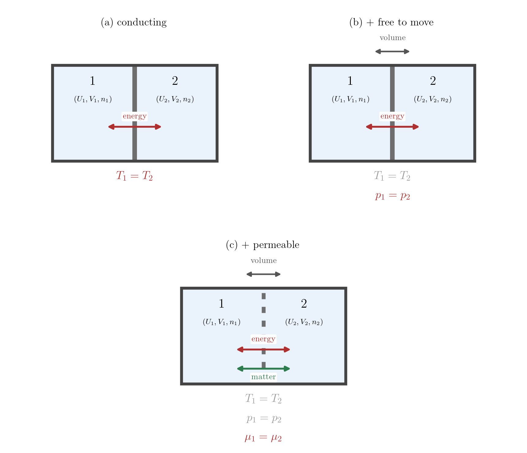
The conditions accumulate as the partition is made more permissive (Figure 8.1): thermal contact equalises the temperature, a movable wall the pressure, a permeable wall the chemical potential. Each is the vanishing of a first derivative of the entropy with respect to the corresponding constraint, and each leans on the equality of temperatures secured by the one before. Together they make precise the intuition that in equilibrium nothing is left that could still flow: no temperature difference to drive a heat flow, no pressure difference to drive a volume change, no difference in chemical potential to drive a matter flow.
These are the first-order conditions, the ones that make the entropy stationary. Because equilibrium is an absolute maximum and not merely a stationary point, it must meet a second-order condition too: the entropy must be concave, so that any transfer across the partition can only lower it. The inequalities this concavity imposes are the stability conditions, to which we now turn.
8.4 Stability
The conditions of the previous section make the entropy stationary, but a stationary point need not be a maximum. Since equilibrium is the absolute maximum, the entropy must in addition be concave: any small redistribution of energy or volume between the parts of the system must lower the total entropy. Were it not so, some fluctuation would raise the entropy, and the system, obeying the law of increase, would run away from the supposed equilibrium instead of returning to it. Concavity is therefore the condition for the equilibrium to be stable, and it makes precise the requirement that the entropy curve downward under any redistribution.
Concavity in the energy and in the volume amounts to two inequalities on measurable quantities, derived in the box below: \[ C_V > 0, \qquad \kappa_T = -\frac{1}{V}\left(\frac{\partial V}{\partial p}\right)_T > 0, \tag{8.12}\] the heat capacity at constant volume \(C_V = (\partial U/\partial T)_V\) (Lecture 3) and the isothermal compressibility are both positive.
These inequalities are the precise content of Le Chatelier’s principle: a system in stable equilibrium answers a disturbance in the sense that opposes it. The restoring tendency is not added by hand; it is the entropy maximum read locally, since concavity makes any fluctuation lower \(S_{\rm tot}\) and the law of increase then drives the fluctuation back. A positive heat capacity means that a region which momentarily takes up a little extra energy grows warmer, and being warmer than its surroundings returns the energy; a positive compressibility means that a region momentarily compressed rises in pressure, and being at higher pressure pushes back out. Each response restores the equilibrium. Should either inequality fail, the corresponding fluctuation would instead be amplified: the equilibrium would be unstable, and the system would break up into regions of different temperature or density.
This is no idle possibility. In Lecture 10 we shall find that a van der Waals isotherm has a range of volumes over which \((\partial p/\partial V)_T > 0\), so that \(\kappa_T < 0\). That branch violates mechanical stability and cannot describe a homogeneous state; it is precisely where the substance separates into liquid and vapour.
Specialise the composite entropy Equation 8.11 to two equal samples of the same substance (so \(n_1 = n_2 = n/2\) and a single entropy function \(S\) serves for both parts), each part keeping its amount of substance fixed, \[ S_{\rm tot}(U_1, V_1) = S(U_1, V_1) + S(U - U_1,\, V - V_1). \] At equilibrium the two parts are in the same state, each holding half of the total, \(U_1 = U_2 = U/2\) and \(V_1 = V_2 = V/2\). Differentiating twice gives \(\partial^2 S_{\rm tot}/\partial U_1^2 = S_{UU}(U_1,V_1) + S_{UU}(U_2,V_2)\), and likewise for the mixed and the volume derivatives; evaluated at the common state these pairs are equal, so the Hessian of \(S_{\rm tot}\) is simply twice the Hessian of the material’s entropy \(S(U,V)\). A factor of two does not change definiteness, so the equilibrium is stable exactly when \(S(U,V)\) is concave: its Hessian must be negative-definite, which for a symmetric \(2\times 2\) matrix holds when the leading entry is negative and the determinant positive,1 \[ S_{UU} < 0, \qquad S_{UU} S_{VV} - S_{UV}^2 > 0, \] with \(S_U = (\partial S/\partial U)_V = 1/T\) and \(S_V = (\partial S/\partial V)_U = p/T\) from Equation 8.3.
Thermal stability. Differentiating \(S_U = 1/T\), \[ S_{UU} = \left(\frac{\partial (1/T)}{\partial U}\right)_V = -\frac{1}{T^2}\left(\frac{\partial T}{\partial U}\right)_V = -\frac{1}{T^2 C_V}, \] so \(S_{UU} < 0\) is exactly \(C_V > 0\).
Mechanical stability. The remaining condition involves the determinant \(S_{UU} S_{VV} - S_{UV}^2\), which is the determinant of the Hessian of \(S(U,V)\) and hence of the Jacobian of its gradient \((S_U, S_V) = (1/T,\, p/T)\) with respect to \((U,V)\). Computing \(S_{VV}\) and \(S_{UV}\) directly would require derivatives taken at constant \(U\), which are awkward; it is far cleaner to change variables from \((U,V)\) to \((T,V)\) and use that the determinant of a Jacobian factorises under composition, \[ \det\frac{\partial(1/T,\, p/T)}{\partial(U,V)} = \det\frac{\partial(1/T,\, p/T)}{\partial(T,V)}\;\det\frac{\partial(T,V)}{\partial(U,V)} . \] The second factor is the Jacobian of the map \((U,V)\mapsto(T,V)\), in which \(V\) maps to itself: \[ \frac{\partial(T,V)}{\partial(U,V)} = \begin{pmatrix} \left(\dfrac{\partial T}{\partial U}\right)_V & \left(\dfrac{\partial T}{\partial V}\right)_U \\[6pt] 0 & 1 \end{pmatrix}, \qquad \det = \left(\frac{\partial T}{\partial U}\right)_V = \frac{1}{C_V}, \] since \((\partial U/\partial T)_V = C_V\). The first factor is \[ \frac{\partial(1/T,\, p/T)}{\partial(T,V)} = \begin{pmatrix} -\dfrac{1}{T^2} & 0 \\[8pt] \dfrac{1}{T}\left(\dfrac{\partial p}{\partial T}\right)_V - \dfrac{p}{T^2} & \dfrac{1}{T}\left(\dfrac{\partial p}{\partial V}\right)_T \end{pmatrix} , \] whose top-right entry vanishes because \(1/T\) depends on \(T\) alone. The matrix is therefore triangular, and its determinant is the product of the diagonal entries, \[ \det\frac{\partial(1/T,\, p/T)}{\partial(T,V)} = \left(-\frac{1}{T^2}\right)\cdot\frac{1}{T}\left(\frac{\partial p}{\partial V}\right)_T = -\frac{1}{T^3}\left(\frac{\partial p}{\partial V}\right)_T . \] Multiplying the two factors gives the determinant of the Hessian, \[ S_{UU} S_{VV} - S_{UV}^2 = -\frac{1}{T^3 C_V}\left(\frac{\partial p}{\partial V}\right)_T . \] With \(C_V > 0\) already established and \(T > 0\), this is positive precisely when \((\partial p/\partial V)_T < 0\), that is when \(\kappa_T > 0\): mechanical stability is the statement that enlarging a region lowers its pressure.
Chemical stability. One might look for a third inequality from the matter direction, on \((\partial\mu/\partial n)\). For a one-component system there is none, and the reason is extensivity. Because \(S(\lambda U, \lambda V, \lambda n) = \lambda S(U, V, n)\), differentiating with respect to \(\lambda\) at \(\lambda = 1\) (Euler) shows that \((U, V, n)\) is a null direction of the Hessian: along it, where the whole system is scaled up at fixed intensive state, \(S\) has no curvature. The full \(3\times 3\) Hessian is therefore singular and can never be strictly negative-definite; the genuine stability conditions live in the two-dimensional space transverse to this scaling direction, and are exactly the \(C_V > 0\) and \(\kappa_T > 0\) found above. Equivalently, for one component \(\mu = \mu(T,p)\) depends on the two intensive variables alone, so \((\partial\mu/\partial n)_{T,p} = 0\): adding matter at fixed \(T\) and \(p\) merely makes more of the same phase. Diffusive stability becomes an independent restriction only for mixtures, where a species’ chemical potential depends on the composition, treated in Lecture 11.
8.5 Summary
For an open system the fundamental relation gains a term, \(dU = T\,dS - p\,dV + \mu\,dn\) (Equation 8.1), which defines the chemical potential \(\mu = (\partial U/\partial n)_{S,V}\) (Equation 8.2), the energy carried in per mole of matter added at fixed entropy and volume. The new term is demanded by energy conservation, and \(\mu\) is intensive. In the entropy representation \((\partial S/\partial n)_{U,V} = -\mu/T\) (Equation 8.4), so the three first derivatives of \(S(U,V,n)\) are the intensive quantities \(1/T\), \(p/T\) and \(-\mu/T\).
For an ideal gas, computed from the definition, \(\mu = u + RT - Ts\) (Equation 8.8), or equivalently \(\mu(T,p) = \mu(T,p_0) + RT\ln(p/p_0)\) (Equation 8.9): the chemical potential rises logarithmically with pressure. This form returns, with \(p\) replaced by a partial pressure, in Lecture 11.
Equilibrium of an isolated system is the absolute maximum of the total entropy \(S_{\rm tot} = S_1 + S_2\) (Equation 8.10) over the internal constraints, at fixed totals. Stationarity yields, as the partition is made successively permeable, \(T_1 = T_2\) (thermal), then \(p_1 = p_2\) (mechanical), then \(\mu_1 = \mu_2\) (diffusive); the first re-derives the Zeroth Law from the Second.
That this stationary point be a maximum, and the equilibrium stable, requires the entropy to be concave: \(C_V > 0\) and \(\kappa_T > 0\) (Equation 8.12), the content of Le Chatelier’s principle. The failure \(\kappa_T < 0\) marks the branch on which a gas separates into liquid and vapour (Lecture 10). For a single component, extensivity leaves no independent diffusive stability condition.
8.6 Problems
Problem 8.1 An ideal gas is compressed isothermally at \(T = 300\ \mathrm{K}\) from pressure \(p_1\) to \(p_2 = 4.0\,p_1\).
Using Equation 8.9, compute the change in chemical potential \(\mu(T, p_2) - \mu(T, p_1)\). (Note that \(\mu\) is intensive, so the result does not depend on the amount of gas.)
The compressed gas is now connected, through a wall permeable to matter and at the same temperature, to a sample of the same gas still at \(p_1\). State in which direction matter flows, and why.
Problem 8.2 An ideal gas expands isothermally at \(T = 350\ \mathrm{K}\) until its density falls to one third of its initial value.
Using Equation 8.9, compute \(\mu(T, p_2) - \mu(T, p_1)\). (At fixed temperature the pressure is proportional to the density.)
Comment on the sign of the result in the light of the fact that matter flows from high to low chemical potential.
Problem 8.3 A system has the entropy, in the entropy representation, \[ S(U, V, n) = n\,s_0 + n\,c_V \ln\frac{U}{n\,u_0} + nR\,\ln\frac{V}{n\,v_0}, \] where \(s_0\), \(u_0\), \(v_0\) and \(c_V\) are constants.
Using the entropy-representation relations \((\partial S/\partial U)_{V,n} = 1/T\), \((\partial S/\partial V)_{U,n} = p/T\) and Equation 8.4, compute the three first derivatives of \(S\) and identify \(1/T\), \(p/T\) and \(-\mu/T\).
Hence show that \(U = n\,c_V T\) and recover the equation of state \(pV = nRT\).
Obtain the chemical potential \(\mu\) as a function of \(T\) and the molar volume \(v = V/n\).
Problem 8.4 A system has the fundamental relation, in the energy representation, \[ U(S, V, n) = n\,u_0 \left(\frac{V}{n\,v_0}\right)^{-R/c_V} \exp\!\left(\frac{S/n - s_0}{c_V}\right), \] with \(u_0\), \(v_0\), \(s_0\) and \(c_V\) constants.
Using Equation 8.1, compute \(T = (\partial U/\partial S)_{V,n}\), \(p = -(\partial U/\partial V)_{S,n}\) and \(\mu = (\partial U/\partial n)_{S,V}\).
Show that \(U = n\,c_V T\) and \(pV = nRT\), recovering the same ideal gas as Problem 8.3; with the same constants \(u_0, v_0, s_0, c_V\) the two fundamental relations are exact inverses.
Verify that \(\mu = (U + pV - TS)/n\). (More demanding.)
Problem 8.5 Two identical bodies, each an incompressible solid of constant heat capacity \(C\) (so its entropy depends on temperature alone, \(dS = C\,dT/T\)), are enclosed together in a rigid, thermally insulated container and brought into contact through a fixed wall that can exchange heat. Initially they are at temperatures \(T_1\) and \(T_2\). (Compare Problem 7.11, which obtained \(T_f\) and \(\Delta S_{\rm tot}\) by integration; here we read them from the entropy maximum and add the stability condition.)
Writing \(U_1\) for the energy of body 1 (with \(U_1 + U_2\) fixed), express the total entropy \(S_{\rm tot}(U_1)\) and show that \(dS_{\rm tot}/dU_1 = 0\) requires the two temperatures to be equal.
Find the common final temperature \(T_f\).
Show that \(d^2 S_{\rm tot}/dU_1^2 < 0\), so the stationary point is a maximum, and that this requires \(C > 0\).
Compute \(\Delta S_{\rm tot}\) and show it is positive for \(T_1 \neq T_2\). (Hint: compare the arithmetic and geometric means of \(T_1\) and \(T_2\).)
Problem 8.6 Like Problem 8.5, but the two bodies have different constant heat capacities \(C_1\) and \(C_2\).
Find the common final temperature \(T_f\) from energy conservation.
Compute \(\Delta S_{\rm tot}\) and verify that it is non-negative.
For \(C_1 = 2 C_2\), \(T_1 = 400\ \mathrm{K}\) and \(T_2 = 300\ \mathrm{K}\), evaluate \(T_f\) and the dimensionless ratio \(\Delta S_{\rm tot}/C_2\) numerically.
Problem 8.7 A rigid, thermally insulated cylinder is divided into two compartments by a frictionless piston that is free to move and can exchange heat, so the two gases may exchange energy and volume but not matter. Each compartment holds \(n\) moles of the same ideal gas (constant molar \(c_V\)). Initially compartment 1 has volume \(V_1^{0}\) and temperature \(T_1^{0}\), compartment 2 has volume \(V_2^{0}\) and temperature \(T_2^{0}\), and the total volume \(V = V_1^{0} + V_2^{0}\) is fixed.
State the equilibrium conditions for the two gases: which intensive variables are equalised, and which is not (Figure 8.1).
Using energy conservation, find the common final temperature \(T_f\), and then the final pressure \(p_f\) and the final volumes.
Compute the total entropy change \(\Delta S_{\rm tot}\).
Problem 8.8 Like Problem 8.7, but compartment 1 holds \(n_1\) moles and compartment 2 holds \(n_2\) moles of the same ideal gas, with \(n_1 \neq n_2\).
Find \(T_f\), the final pressure \(p_f\), and the final volumes \(V_{1f}\), \(V_{2f}\).
Show that the final volumes satisfy \(V_{1f}/V_{2f} = n_1/n_2\), and interpret.
For \(n_1 = 1.0\ \mathrm{mol}\), \(T_1^{0} = 300\ \mathrm{K}\), \(n_2 = 2.0\ \mathrm{mol}\), \(T_2^{0} = 450\ \mathrm{K}\) and \(V = 30\ \mathrm{L}\), evaluate \(T_f\), \(p_f\), \(V_{1f}\) and \(V_{2f}\).
Problem 8.9 (More demanding.) This problem fills in the thermal-stability step of the stability box.
Starting from \((\partial S/\partial U)_{V,n} = 1/T\), show that the curvature \((\partial^2 S/\partial U^2)_{V,n} = -1/(T^2 C_V)\), so that the concavity condition \((\partial^2 S/\partial U^2)_{V,n} < 0\) is equivalent to \(C_V > 0\).
Consider two halves of such a system, in contact through a wall that can exchange heat, and suppose that over some range \(C_V < 0\). Show that a small transfer of energy from one half to the other then raises the total entropy, so the uniform state is not a maximum. State what the system does instead.
Problem 8.10 (More demanding. Forward-looking: previews Lecture 10.) This problem fills in the mechanical-stability step of the stability box.
The Hessian of \(S(U, V)\) (at fixed \(n\)) has determinant \(S_{UU} S_{VV} - S_{UV}^2\). By changing variables from \((U, V)\) to \((T, V)\), show that, given \(C_V > 0\), the condition \(S_{UU} S_{VV} - S_{UV}^2 > 0\) reduces to \((\partial p/\partial V)_T < 0\), that is \(\kappa_T > 0\).
Suppose that along one isotherm a fluid has a stretch of volumes over which \((\partial p/\partial V)_T > 0\). Explain why no homogeneous state can exist there, and what the fluid does instead.
Problem 8.11 (More demanding.) For a one-component system the entropy \(S(U, V, n)\) is extensive, \(S(\lambda U, \lambda V, \lambda n) = \lambda S(U, V, n)\) for all \(\lambda > 0\).
Differentiate this relation with respect to \(\lambda\) and set \(\lambda = 1\) to obtain the Euler relation \(U\,S_U + V\,S_V + n\,S_n = S\).
Differentiate again to show that the Hessian of \(S\) has \((U, V, n)\) as a null direction, so the \(3 \times 3\) Hessian is singular.
Conclude that a one-component system has no independent diffusive stability condition beyond \(C_V > 0\) and \(\kappa_T > 0\), and interpret the null direction physically.
Problem 8.12 (More demanding. Forward-looking: previews Lecture 11.)
For a one-component system the chemical potential depends only on \(T\) and \(p\). Use this to argue that \((\partial \mu/\partial n)_{T,p} = 0\), and explain why adding matter at fixed temperature and pressure simply produces more of the same phase.
In a mixture of two species the chemical potential of each depends also on the composition. For an ideal mixture, \(\mu_i\) rises with the mole fraction \(x_i = n_i/n\) of species \(i\). Explain why \((\partial \mu_i/\partial n_i)_{T,p} > 0\) is then a genuine diffusive stability condition, in contrast to the one-component case of part (a).
Problem 8.13 (Forward-looking: previews Lecture 10.) A liquid and its vapour, a single substance, coexist at temperature \(T\) and pressure \(p\).
From the diffusive equilibrium condition of Figure 8.1, state the relation between the chemical potentials of the two phases.
Model the vapour as an ideal gas, so \(\mu_{\rm vap}(T, p) = \mu_{\rm vap}(T, p_0) + RT \ln(p/p_0)\) (Equation 8.9), and take the chemical potential of the liquid to be essentially independent of pressure, \(\mu_{\rm liq}(T, p) \approx \mu_{\rm liq}(T)\). Show that the coexistence pressure satisfies \[ \ln\frac{p}{p_0} = \frac{\mu_{\rm liq}(T) - \mu_{\rm vap}(T, p_0)}{RT}. \]
If the numerator has the form \(\mu_{\rm liq}(T) - \mu_{\rm vap}(T, p_0) = -L_0 + c\,T\) with \(L_0 > 0\) and \(c\) constants, find \(p(T)\) and sketch its temperature dependence.
Problem 8.14 (Forward-looking: previews Lecture 10.) Like Problem 8.13, for the coexistence of a solid with its vapour (sublimation).
Write the coexistence condition \(\mu_{\rm sol}(T) = \mu_{\rm vap}(T, p)\), again treating the vapour as ideal and the solid’s chemical potential as pressure-independent.
Taking \(\mu_{\rm sol}(T) - \mu_{\rm vap}(T, p_0) = -L_{\rm s} + c_{\rm s} T\), find the sublimation pressure \(p(T)\).
Given \(L_{\rm s} = 5.0 \times 10^4\ \mathrm{J\,mol^{-1}}\), \(c_{\rm s} = 0\) and \(p_0 = 1.0 \times 10^5\ \mathrm{Pa}\), evaluate the ratio \(p(250\ \mathrm{K})/p(200\ \mathrm{K})\).
A symmetric matrix is negative-definite when its leading principal minors alternate in sign, beginning with a negative one; for a \(2\times 2\) matrix this means a negative leading entry and a positive determinant. This is Sylvester’s criterion.↩︎