10 Phase Transitions
Part IV — Phase Transitions and Chemical Equilibrium
Last updated: 30-06-2026
10.1 Where this lecture is going
Water boils and ice melts at sharp temperatures, ice and water and vapour coexist at one triple point, and a gas will not liquefy under any pressure unless it is first cooled below a certain temperature. Two questions run through all of these: at a given \(T\) and \(p\), which phase is realised, and when do two phases coexist?
One principle answers both. At fixed \(T\) and \(p\) a system settles where its Gibbs free energy \(G\) is least; offered several phases, each with its own chemical potential \(\mu(T,p)\), the substance takes the one of lowest \(\mu\), and where two are equal those phases coexist. Equal temperature and equal pressure are already secured by thermal and mechanical equilibrium, so the single new condition is this equality of chemical potentials.
We develop this generally first, then for one component: the framework for any number of phases and species, with \(G\) minimised to give the equilibrium conditions and the Gibbs phase rule; then the one-component phase diagram, the latent heat of a first-order transition, the Clausius–Clapeyron relation, and the van der Waals loop with its Maxwell construction and critical point.
10.2 Phases, species, and the Gibbs free energy
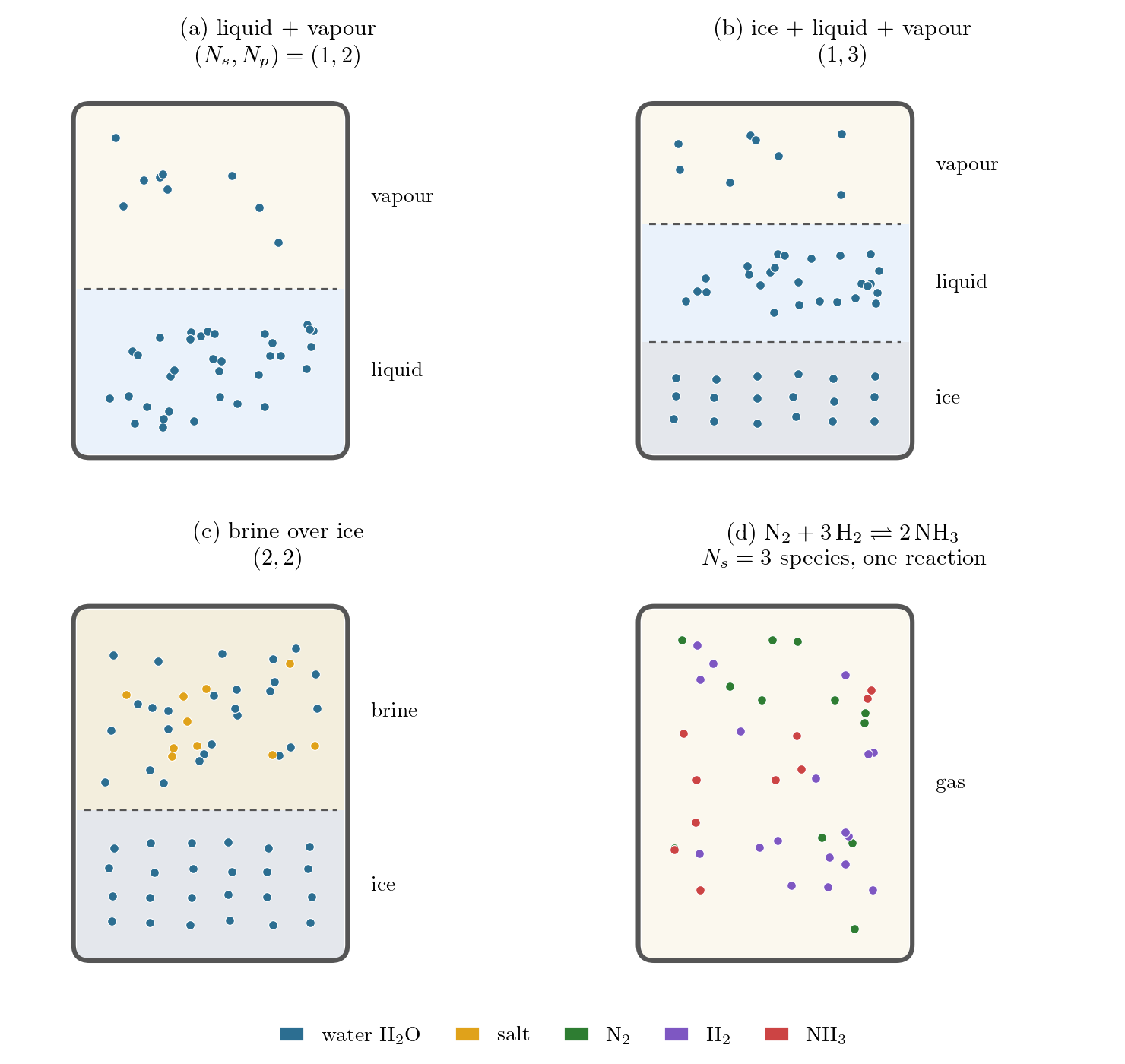
A phase transition involves more than one homogeneous body at once. The simplest case is ice floating in water: one substance present as two phases, solid and liquid, sharing a common temperature and pressure while matter passes between them. We shall want the general setting as well, a liquid beneath its own vapour or several solids freezing out of a melt, so we widen the system from the start. Let it contain \(N_s\) chemical species, the molecular constituents, indexed \(i = 1, \dots, N_s\), distributed among \(N_p\) phases, indexed \(\alpha = 1, \dots, N_p\). A phase is a homogeneous region of the system, uniform in temperature, pressure and composition, though not necessarily of a single species: phase \(\alpha\) holds \(n_{\alpha,i}\) moles of species \(i\), and the state of the whole is fixed by \(T\), \(p\) and the array \(\{n_{\alpha,i}\}\). Four examples, of growing generality, are gathered in Figure 10.1.
Phase — a homogeneous region of the system, uniform in \(T\), \(p\) and composition. The liquid, the solid and the vapour of a substance are distinct phases.
We treat throughout one particular, and physically the most common, arrangement. The whole system is closed: no matter crosses its outer boundary, only heat and work. The matter inside is free to redistribute, though, moving from one phase to another (and, where species react, from one species to another), so each phase, taken by itself, is an open subsystem. The phases are in thermal and mechanical contact, with one another and with the surroundings. Two bodies in thermal contact share, at equilibrium, a single temperature: this is thermal equilibrium, the content of the Zeroth Law and the very definition of temperature of Lecture 3. Across a movable, frictionless boundary the forces balance only when the pressures are equal: mechanical equilibrium. A single temperature \(T\) and a single pressure \(p\) therefore describe all the phases at once, equal to those of the surroundings (\(p_{\rm ext} = p\)). Neither equality is special to phase transitions or assumed for convenience; both have been in hand since the foundations of the course. The one equilibrium still to be located, and the subject of this lecture, is the diffusive equilibrium: how matter distributes among the phases, settled in the next section by minimising the Gibbs free energy \(G\).
Each phase is an open subsystem, and its internal energy obeys the fundamental relation in the open-system form of Lecture 8, now carrying one chemical-potential term for each species present. For an infinitesimal process between neighbouring equilibrium states, \[ dU_\alpha = T\,dS_\alpha - p\,dV_\alpha + \sum_i \mu_{\alpha,i}\,dn_{\alpha,i}, \tag{10.1}\] in which \(\mu_{\alpha,i} = (\partial U_\alpha/\partial n_{\alpha,i})_{S_\alpha, V_\alpha,\, n_{\alpha,j\neq i}}\) is the energy carried in by one mole of species \(i\) added to phase \(\alpha\) at fixed entropy, volume and other amounts: the chemical potential of that species in that phase.
Chemical potential \(\mu_{\alpha,i}\) — intensive; the energy per mole to add species \(i\) to phase \(\alpha\) at fixed \(S_\alpha\), \(V_\alpha\) and the other amounts.
The internal energy of a phase is extensive in all of its arguments, and that extensivity does more than shape the differential Equation 10.1: as in Lecture 9, it fixes the value of the energy itself. Scaling a phase up means multiplying \(S_\alpha\), \(V_\alpha\) and every amount \(n_{\alpha,i}\) by one common factor, leaving the composition and the intensive state unchanged; first-order homogeneity then gives the Euler relation \[ U_\alpha = T S_\alpha - p V_\alpha + \sum_i \mu_{\alpha,i}\,n_{\alpha,i}, \tag{10.2}\] the natural generalisation of the one-component \(U = TS - pV + \mu n\) of Lecture 9 (the proof is in the box below). The Gibbs free energy of the phase is \(G_\alpha = U_\alpha - T S_\alpha + p V_\alpha\), and its differential, by the same Legendre step as in Lecture 9, \[ dG_\alpha = -S_\alpha\,dT + V_\alpha\,dp + \sum_i \mu_{\alpha,i}\,dn_{\alpha,i}, \tag{10.3}\] identifies each chemical potential as a partial molar Gibbs free energy, the derivative \(\mu_{\alpha,i} = (\partial G_\alpha/\partial n_{\alpha,i})_{T,p,\,n_{\alpha,j\neq i}}\). The Euler relation then gives the value of \(G_\alpha\) itself, each species’ amount weighted by its partial molar value, \[ G_\alpha = \sum_i n_{\alpha,i}\,\mu_{\alpha,i}. \tag{10.4}\] The total Gibbs free energy is additive over the phases: \(U\), \(S\) and \(V\) each add over the spatially distinct phases, so at the common \(T\) and \(p\), \[ G(T,p,\{n_{\alpha,i}\}) = \sum_\alpha G_\alpha . \tag{10.5}\] Read physically, the Gibbs free energy of a phase is its content of each species weighted by what that species is worth per mole, its partial molar Gibbs free energy \(\mu_{\alpha,i}\) (equal to the whole molar value \(G_\alpha/n_\alpha\) only when the phase is a single species, as in Lecture 9).
Euler relation \(U_\alpha = TS_\alpha - pV_\alpha + \sum_i \mu_{\alpha,i} n_{\alpha,i}\) — the finite relation extensivity forces, fixing the value of a phase’s energy, not just its differential.
That a phase is extensive means scaling it at fixed intensive state multiplies its extensive variables together: picturing \(\lambda\) identical copies of phase \(\alpha\) merged into one larger phase at the same \(T\), \(p\) and chemical potentials, \[ U_\alpha(\lambda S_\alpha, \lambda V_\alpha, \{\lambda n_{\alpha,i}\}) = \lambda\,U_\alpha(S_\alpha, V_\alpha, \{n_{\alpha,i}\}), \qquad \lambda > 0, \] so \(U_\alpha\) is a first-order homogeneous function of its extensive arguments. Differentiating both sides with respect to \(\lambda\) and setting \(\lambda = 1\) (Euler’s theorem on homogeneous functions, exactly the step taken for one component in Lecture 9, now with several \(n_{\alpha,i}\)), \[ S_\alpha\left(\frac{\partial U_\alpha}{\partial S_\alpha}\right)_{V_\alpha,\,\{n\}} + V_\alpha\left(\frac{\partial U_\alpha}{\partial V_\alpha}\right)_{S_\alpha,\,\{n\}} + \sum_i n_{\alpha,i}\left(\frac{\partial U_\alpha}{\partial n_{\alpha,i}}\right)_{S_\alpha,V_\alpha,\,n_{\alpha,j\neq i}} = U_\alpha . \] Reading the three derivatives off Equation 10.1 as \(T\), \(-p\) and \(\mu_{\alpha,i}\) returns the Euler relation Equation 10.2.
10.3 Equilibrium minimises the Gibbs free energy
Lecture 9 established that a single phase, held at the temperature and pressure of its surroundings, comes to rest where its Gibbs free energy is least. That bound carries over to the present system unchanged; only the free coordinate is new, the distribution of matter among the phases.
Let the system relax from an initial state that is not yet the equilibrium one. There each phase is homogeneous, with a definite composition, and shares the common temperature \(T\) and pressure \(p\) of the surroundings, so \(U\), \(S\), \(V\) and hence \(G = \sum_\alpha G_\alpha\) are all well defined. What has not yet settled is the distribution of matter \(\{n_{\alpha,i}\}\), still free to change by transfer of a species between phases and, where species react, by interconversion within a phase. The system then evolves to its true equilibrium, again at the surroundings’ \(T\) and \(p\). The whole system being closed, its energy balance over this evolution is the ordinary first law \(\Delta U = Q - W\), with the boundary work \(W = p_{\rm ext}\,\Delta V = p\,\Delta V\) (the boundary is frictionless) and the heat it absorbs bounded by the Clausius inequality \(Q \le T_{\rm res}\,\Delta S = T\,\Delta S\) (Lecture 7). Since both endpoints sit at the surroundings’ \(T\) and \(p\), the right-hand side of \(\Delta U \le T\,\Delta S - p\,\Delta V\) is \(\Delta(TS) - \Delta(pV)\), so that \[ \Delta(U - TS + pV) = \Delta G \le 0 \qquad (\text{constant } T, p), \tag{10.6}\] with equality only in the reversible limit. The Gibbs free energy can thus only fall as the system approaches equilibrium, and equilibrium at constant \(T\) and \(p\) is the state of least \(G\): the bound of Lecture 9 (Equation 9.12), unchanged.
What is new is the coordinate over which \(G\) is minimised. Because \(G = \sum_\alpha G_\alpha\) (Equation 10.5) is defined for any matter distribution \(\{n_{\alpha,i}\}\), not the equilibrium one alone, the bound (Equation 10.6) says the equilibrium is the distribution of least \(G\) among all those the system can reach by redistributing its matter internally. Thermal and mechanical equilibrium having already fixed the common \(T\) and \(p\), the distribution \(\{n_{\alpha,i}\}\) is the freedom that remains, and the next section minimises \(G\) over it to read off the conditions of equilibrium.
10.4 The equilibrium conditions and the phase rule
At the common \(T\) and \(p\) the matter is free to move, and equilibrium is the arrangement of least \(G\). Two kinds of move are open to it: a species may pass from one phase to another, or, where the chemistry allows, species may interconvert by a reaction. Whichever occurs, the mole numbers change by some \(\{dn_{\alpha,i}\}\); since \(G = \sum_\alpha G_\alpha\) with each phase obeying its Gibbs differential Equation 10.3, at fixed \(T\) and \(p\) \[ dG = \sum_{\alpha,i} \mu_{\alpha,i}\,dn_{\alpha,i} \qquad (\text{fixed } T, p). \tag{10.7}\] The chemical potentials are the prices that drive the rearrangement, and equilibrium is where no permitted move can lower \(G\), that is, where this vanishes for every change the constraints allow. The constraint is conservation: matter is only moved, never created, so the amount of each element is fixed. With no reactions present that is simply each species’ total, \(\sum_\alpha n_{\alpha,i} = n_i\).
Phase equilibrium. Take the simplest move, carrying \(dn\) moles of species \(i\) from phase \(\beta\) into phase \(\alpha\) (\(dn_{\alpha,i} = +dn\), \(dn_{\beta,i} = -dn\), all else held): the equal and opposite changes leave the total \(n_i\) fixed, so the move is allowed. Only two terms of Equation 10.7 survive, and \(dG = (\mu_{\alpha,i} - \mu_{\beta,i})\,dn\). At a minimum \(dG\) cannot be negative for either sign of \(dn\), for if the bracket were nonzero one sign would lower \(G\); it must therefore vanish: \[ \mu_{\alpha,i} = \mu_{\beta,i} \tag{10.8}\] for each species \(i\) and every pair of phases in which it is present. The chemical potential of each species thus takes the same value in every phase it occupies. This is the diffusive-equilibrium condition \(\mu_1 = \mu_2\) of Lecture 8, obtained there by maximising the entropy of an isolated system and recovered here by minimising \(G\) at fixed \(T\) and \(p\): one physical condition, read off whichever potential the constraints make natural.
Reaction equilibrium. When species interconvert their mole numbers are no longer independent. A reaction consumes and produces species in fixed whole-number proportions, its stoichiometric coefficients \(\nu_i\): for \(2\,\mathrm{H_2} + \mathrm{O_2} \rightarrow 2\,\mathrm{H_2O}\) they are \(-2, -1, +2\), counted negative for a species consumed and positive for one produced. The whole reaction advances together by a single number, its extent \(\xi\), so \(dn_i = \nu_i\,d\xi\). The reaction runs within a phase, where the chemical potentials carry no phase label (Equation 10.8); substituted into Equation 10.7, this gives \(dG = \big(\sum_i \nu_i \mu_i\big)\,d\xi\), so a stationary \(G\) requires \(\sum_i \nu_i \mu_i = 0\). We name the condition here and put it to work in Lecture 11; for the rest of this lecture no reactions occur.
The Gibbs phase rule. How much freedom does coexistence leave? The count that decides it is the number of independent components, \(N_c = N_s - N_r\): the \(N_s\) species less the \(N_r\) independent reactions that link them, so with no reactions \(N_c = N_s\). (The ammonia mixture of Figure 10.1, three species joined by one reaction, has \(N_c = 2\).) Now set the intensive variables that fix the state of every phase against the equilibrium conditions (Equation 10.8): each phase carries \(N_c - 1\) independent composition fractions, the common \(T\) and \(p\) add two, and those conditions remove \(N_c(N_p - 1)\). The balance is the variance \[ f = N_c - N_p + 2 , \tag{10.9}\] the number of intensive variables one may still vary freely while keeping all \(N_p\) phases in coexistence. For a pure substance (\(N_c = 1\)) it reads \(f = 3 - N_p\): a single phase fills a two-dimensional region of the \((T,p)\) plane (\(f = 2\)), two phases coexist only along a curve (\(f = 1\)), and three meet at one isolated triple point (\(f = 0\)). No more than three phases of a single substance can coexist. The sections that follow trace out exactly this structure.
Component — a species whose amount can be varied independently of the others. Their number \(N_c = N_s - N_r\) is the species count less the \(N_r\) independent reactions, since each reaction removes one degree of freedom from the composition.
The intensive state of the assembly is fixed by \(T\), \(p\), and the composition of every phase. A phase of \(N_s\) species has \(N_s\) mole fractions constrained to sum to one, hence \(N_s - 1\) independent; across \(N_p\) phases that is \(N_p(N_s - 1)\) composition variables, and with \(T\) and \(p\), \[ \#\text{variables} = 2 + N_p(N_s - 1). \] The equalities cut this down. For each species the equal-potential condition (Equation 10.8) supplies \(N_p - 1\) independent equations, and so \(N_s(N_p - 1)\) in all; the \(N_r\) reaction conditions \(\sum_i \nu_i \mu_i = 0\) add \(N_r\) more. Subtracting, \[ f = \big[2 + N_p(N_s - 1)\big] - \big[N_s(N_p - 1) + N_r\big] = (N_s - N_r) - N_p + 2 = N_c - N_p + 2 . \] The count takes every species to be present in every phase: a species absent from one phase drops a variable (its fraction there) and an equality (its balance against that phase) together, leaving \(f\) untouched. Any further constraint, a fixed composition ratio or electroneutrality, lowers \(f\) by one.
10.5 One component: coexistence and the phase diagram
The rest of the lecture takes the simplest case, a single substance: one species, \(N_c = 1\), so only the phase index survives and the equilibrium condition (Equation 10.8) becomes \(\mu_1 = \mu_2\) between any two phases. For one component the chemical potential of a phase is nothing but its molar Gibbs free energy, \(\mu_\alpha(T,p) = G_\alpha/n_\alpha\) (Equation 9.14), a function of \(T\) and \(p\) alone. Held at fixed \(T\) and \(p\) and free to choose its phase, the substance minimises \(G = n\mu\) by sitting entirely in whichever phase offers the lowest \(\mu(T,p)\). Two phases share the substance only where their chemical potentials are equal, \[ \mu_1(T,p) = \mu_2(T,p). \tag{10.10}\]
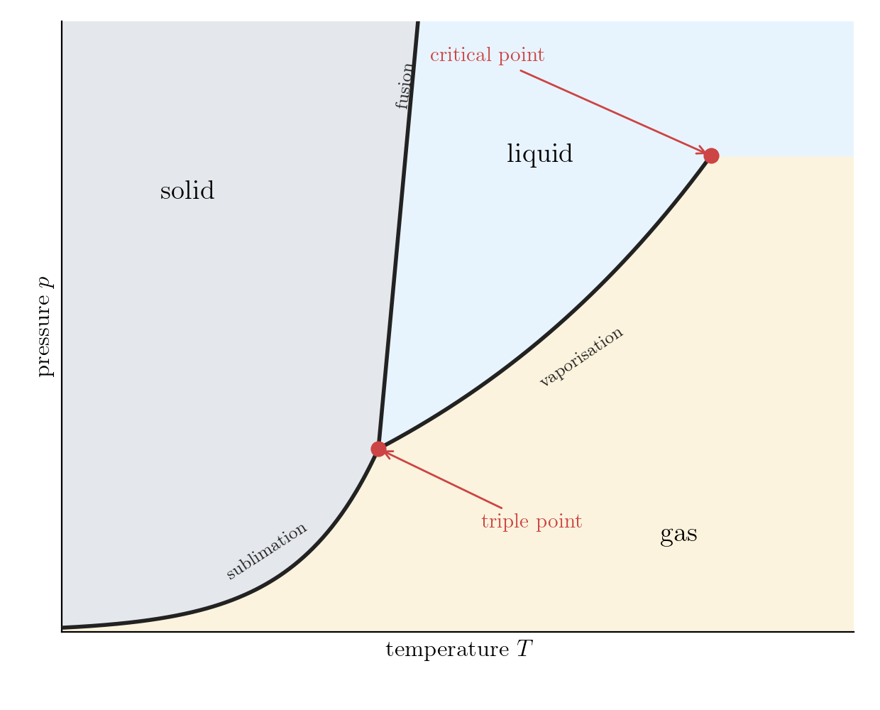
One equation in the two unknowns \(T\) and \(p\) leaves one direction free: its solutions form a whole coexistence curve \(p(T)\) in the plane, the locus \(\mu_1 = \mu_2\) along which two phases share the substance, and the one freedom the phase rule allotted them. Off the curve one phase has the lower \(\mu\) and wins outright, so the plane divides into single-phase regions, solid, liquid and vapour; the map of these regions and the curves between them is the substance’s phase diagram (Figure 10.2). Nothing in Equation 10.10 fixes how the matter splits between two coexisting phases: that proportion is set instead by the heat or volume the surroundings impose. This is why melting and boiling proceed at a fixed temperature while heat flows, as the next section makes precise.
Add a third phase and a second equation joins the first: \(\mu_1 = \mu_2 = \mu_3\) pins both unknowns, so the solid, liquid and vapour of a pure substance meet only at a single isolated triple point, the three-phase limit the phase rule already set. One of these curves is special: the liquid–vapour line does not run on without end but terminates at a critical point, beyond which liquid and gas cease to be distinct and the one passes smoothly into the other. The closing section traces how the van der Waals isotherm produces it.
10.6 First-order transitions and latent heat
What becomes of the chemical potential as the substance crosses a coexistence curve? On the curve the two phases share it, \(\mu_1 = \mu_2\), and on either side the substance follows whichever branch lies lower, so the physical \(\mu\) joins continuously across the curve. Its slope need not. The molar Gibbs–Duhem relation \(d\mu = -s\,dT + v\,dp\) (Equation 9.5) reads the first derivatives of \(\mu\) as the molar entropy and volume, \[ s = -\left(\frac{\partial \mu}{\partial T}\right)_p, \qquad v = \left(\frac{\partial \mu}{\partial p}\right)_T, \tag{10.11}\] and these the two phases do not share: vapour is far less dense than the liquid it rises from (so \(v\) differs), and the more ordered phase carries the lower entropy (so \(s\) differs). So while \(\mu\) joins continuously, its slopes jump, \(\Delta s = s_2 - s_1 \neq 0\) and \(\Delta v = v_2 - v_1 \neq 0\), leaving a corner in \(\mu(T,p)\) where the lower branch changes hands (Figure 10.3). Because the first derivatives of \(\mu\) are the lowest to be discontinuous, such a transition is called first-order.
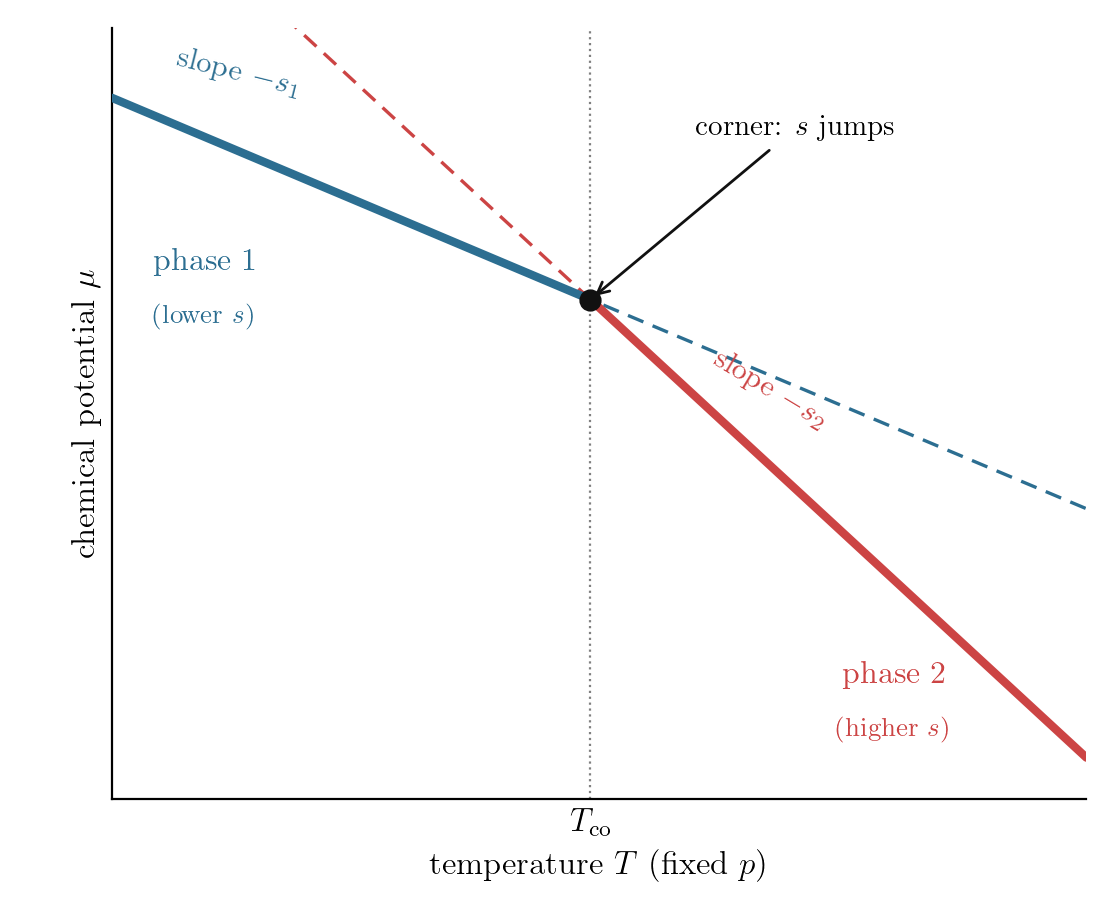
Because the phases differ in entropy, converting between them exchanges heat. Take one mole from phase 1 to phase 2 at the fixed \(T\) and \(p\) of the curve: its entropy changes by \(\Delta s\), and since the phases are in equilibrium the conversion is reversible, so the heat absorbed is \(T\,\Delta s\), the latent heat \[ L = T\,\Delta s = T(s_2 - s_1) , \tag{10.12}\] with phase 2 the higher-entropy phase, so that \(L > 0\) is the heat absorbed on heating. It is taken up phase by phase with the thermometer standing still: the heat that melts ice or boils water yet raises no temperature until the last of the old phase is gone.
Not every transition is of this kind. Where instead the molar entropy and volume join smoothly too, so that \(\Delta s\) and \(\Delta v\) vanish and no latent heat is exchanged, the transition is continuous, any singularity appearing only in a higher derivative such as the heat capacity. The critical point ending the liquid–vapour curve is such a transition: there the two phases become identical, and we meet it again where the van der Waals isotherm flattens in the closing section.
10.7 The Clausius–Clapeyron relation
The coexistence curve is, by definition, the locus of states \((T,p)\) at which \(\mu_1(T,p) = \mu_2(T,p)\), so the equality holds not at an isolated point but identically along the whole curve. A displacement \((dT, dp)\) that stays on the curve must therefore preserve it, changing the two chemical potentials by equal amounts, \(d\mu_1 = d\mu_2\). Writing each with the molar Gibbs–Duhem relation \(d\mu_\alpha = -s_\alpha\,dT + v_\alpha\,dp\) gives \(-s_1\,dT + v_1\,dp = -s_2\,dT + v_2\,dp\), and collecting terms leaves the slope of the curve, the Clausius–Clapeyron relation \[ \frac{dp}{dT} = \frac{s_2 - s_1}{v_2 - v_1} = \frac{L}{T\,\Delta v} , \tag{10.13}\] the last step using \(L = T\,\Delta s\) (Equation 10.12). The steepness of a coexistence curve is fixed entirely by the latent heat and the volume change of the transition, both of them measurable. (The same slope was reached by a Carnot argument in Problem 9.9.)
For the liquid–vapour line two simplifications put the relation in a form we can integrate. The molar volume of the liquid is negligible beside that of the vapour, so \(\Delta v \approx v_{\rm gas}\), and the vapour, being dilute, is nearly ideal, \(v_{\rm gas} = RT/p\). The relation becomes \[ \frac{d\ln p}{dT} = \frac{L}{R T^2} \;\Longrightarrow\; p(T) = p_0\,\exp\!\left[-\frac{L}{R}\left(\frac1T - \frac1{T_0}\right)\right] , \tag{10.14}\] the integration taking \(L\) roughly constant over the range. This is the vapour-pressure curve: the saturated vapour pressure rises steeply with temperature. It rests on three approximations, each worth keeping in sight, \(v_{\rm liquid} \ll v_{\rm gas}\), an ideal vapour, and a constant \(L\); the curve and these steps are built up in Problem 8.13.
Putting in numbers, the relation sets a scale. For water boiling at \(T = 373\ \mathrm{K}\), with \(L \approx 41\ \mathrm{kJ\,mol^{-1}}\), it gives \(dp/dT = Lp/(RT^2) \approx 3.6\ \mathrm{kPa\,K^{-1}}\). Atmospheric pressure falls by about \(12\ \mathrm{Pa}\) for every metre climbed (roughly \(\rho_{\rm air}\,g\)), so near sea level the boiling point drops by about \(1\ \mathrm{K}\) for every \(300\ \mathrm{m}\) of ascent; on the highest summits, some nine kilometres up, water boils near \(70\,^{\circ}\mathrm{C}\).
One substance runs the other way. Ice is less dense than the water it melts into, so \(\Delta v = v_{\rm liquid} - v_{\rm solid} < 0\) across the solid–liquid line; with \(L > 0\) still, Equation 10.13 then makes \(dp/dT < 0\): the melting curve of water leans backward, so that raising the pressure lowers the melting point. The reversed sign is rare, and it traces to the open, low-density structure of ice.
10.8 The van der Waals isotherms: tie-line, Maxwell construction, critical point
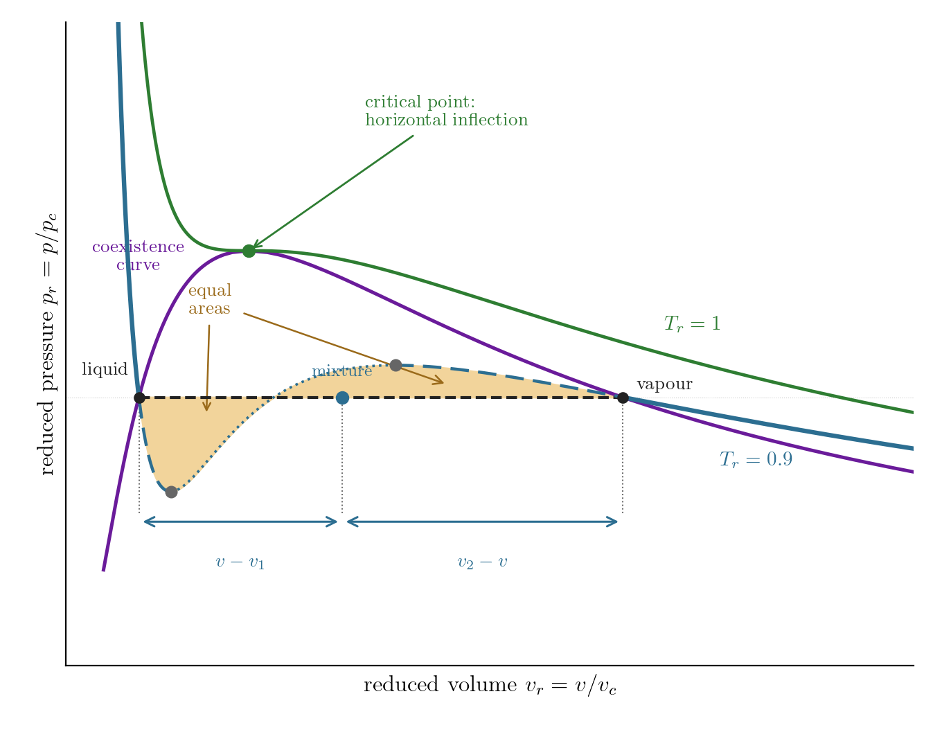
The coexistence condition \(\mu_1 = \mu_2\) tells us that two phases can meet, but not at what pressure nor with what volumes. To pin those down we need a concrete equation of state, and the van der Waals gas (Problem 9.1, written here per mole) supplies a simple analytic one. Below the critical temperature its isotherm is not monotonic but S-shaped in the \((v,p)\) plane (Figure 10.4): as the volume grows the pressure first falls steeply (the stiff liquid), then rises over a middle stretch, then falls again (the vapour). A single pressure can be met at three volumes.
The rising stretch cannot be a stable state. On it \((\partial p/\partial v)_T > 0\), so the isothermal compressibility \(\kappa_T = -v^{-1}(\partial v/\partial p)_T\) is negative: squeeze the substance and it would push back less, not more. Stability forbids this (Equation 8.12), and the segment between the two spinodal points, where \((\partial p/\partial v)_T = 0\), is mechanically unstable. The arcs just outside the spinodals still have \(\kappa_T > 0\) and are locally stable, yet they do not carry the lowest \(\mu\), and so are only metastable: the superheated liquid and supercooled vapour seen when a clean, undisturbed sample is carried past its transition.
What the substance actually does is replace the whole loop by a horizontal tie-line at a pressure \(p_*(T)\), running from a liquid end at \(v_1\) to a vapour end at \(v_2\), the two in coexistence at \(\mu_1 = \mu_2\). That equality fixes \(p_*\). The chemical potential is a smooth function of the analytic equation of state all along the isotherm, defined even on the forbidden branch, and at constant \(T\) the molar Gibbs–Duhem relation reads \(d\mu = v\,dp\); integrating from one stable end to the other, \[ \mu_2 - \mu_1 = \int_1^2 v\,dp = 0 . \tag{10.15}\] Because both ends sit at the same pressure \(p_*\), this integral has a clean geometric meaning: the tie-line must cut the loop so that the two lobes it encloses, above and below, have equal area. This is the Maxwell equal-area construction, the condition \(\mu_1 = \mu_2\) drawn straight onto the isotherm; the integration by parts behind it is in the box.
With both ends at the common pressure \(p_*\), integrate Equation 10.15 by parts: \[ \int_1^2 v\,dp = \big[\,p\,v\,\big]_1^2 - \int_1^2 p\,dv = p_*(v_2 - v_1) - \int_1^2 p\,dv = 0, \] so \(\int_1^2 p\,dv = p_*(v_2 - v_1)\). On the left is the area under the isotherm between the two ends; on the right, the area of the rectangle under the tie-line. Their equality means the loop’s bulge above the tie-line and its dip below it enclose the same area: the two lobes match.
A point on the tie-line, at a molar volume \(v\) between \(v_1\) and \(v_2\), is not a single phase but a mixture of the two. With \(x_1\) and \(x_2\) the mole fractions of liquid and vapour, conservation of matter and of volume, \(x_1 + x_2 = 1\) and \(x_1 v_1 + x_2 v_2 = v\), gives the lever rule \[ \frac{x_2}{x_1} = \frac{v - v_1}{v_2 - v} , \tag{10.16}\] so the amount of each phase is proportional to the tie-line segment reaching across to the other phase: the vapour fraction \(x_2\) to \(v - v_1\), the distance from the liquid end, and the liquid fraction \(x_1\) to \(v_2 - v\), the distance from the vapour end. Near the liquid end the mixture is almost all liquid, near the vapour end almost all vapour.
As \(T\) rises toward \(T_c\) the loop shrinks and the tie-line with it, its two ends drawing together until \(\Delta v \to 0\) and \(\Delta s \to 0\). At \(T_c\) they merge: the first-order line ends and the transition becomes continuous, the critical point where the liquid–vapour curve stops (Figure 10.2). There the S-shape has flattened to a single horizontal inflection, \[ \left(\frac{\partial p}{\partial v}\right)_{T} = \left(\frac{\partial^2 p}{\partial v^2}\right)_{T} = 0 . \tag{10.17}\] Solving these two conditions for the van der Waals constants (Problem 9.1, per mole, gives \(v_c = 3b\), \(T_c = 8a/27Rb\), \(p_c = a/27b^2\)) leaves a pure number, free of \(a\) and \(b\), \[ \frac{p_c\, v_c}{R T_c} = \frac{3}{8} . \tag{10.18}\] Measured in units of their critical values, every van der Waals gas then obeys one and the same reduced equation of state, the dimensionless form Problem 9.1 derives: a law of corresponding states, the kind of universality already met in Carnot’s theorem (Section 6.1), where one result held for every working substance.
10.9 Summary
- The closed system holds \(N_s\) species in \(N_p\) phases at a common \(T\) and \(p\) (thermal and mechanical equilibrium); its Gibbs free energy is additive, \(G = \sum_\alpha G_\alpha\) (Equation 10.5), and at fixed \(T, p\) equilibrium is the matter distribution of least \(G\) (Equation 10.6).
- Minimising \(G\) adds the diffusive conditions: phase equilibrium \(\mu_{\alpha,i} = \mu_{\beta,i}\) (Equation 10.8) and, where species react, reaction equilibrium \(\sum_i \nu_i \mu_i = 0\) (developed in Lecture 11). Counting intensive freedoms against these equalities gives the Gibbs phase rule \(f = N_c - N_p + 2\), with \(N_c = N_s - N_r\) components (Equation 10.9).
- One component (\(f = 3 - N_p\)) has single-phase regions, coexistence curves where \(\mu_1 = \mu_2\) (Equation 10.10), an isolated triple point, and a critical point ending the liquid–vapour curve.
- Across a coexistence curve \(\mu\) is continuous but \(s\) and \(v\) jump, a first-order transition, the entropy jump carried as latent heat \(L = T\,\Delta s\) (Equation 10.12). The curve’s slope is Clausius–Clapeyron, \(dp/dT = \Delta s/\Delta v = L/(T\,\Delta v)\) (Equation 10.13), integrating for liquid–vapour to \(p \propto \exp(-L/RT)\).
- The van der Waals isotherm locates coexistence: its unstable rising branch (\(\kappa_T < 0\)) gives way to a tie-line fixed by the Maxwell equal-area construction \(\int_1^2 v\,dp = 0\) (Equation 10.15), with mixtures split by the lever rule (Equation 10.16). At the critical point the transition turns continuous and \(p_c v_c / R T_c = 3/8\) for every such gas (corresponding states; Problem 9.1).
10.10 Problems
Problem 10.1 Use the Gibbs phase rule \(f = N_c - N_p + 2\) (Equation 10.9) to find the variance in each case.
A pure substance present as a single phase; as two phases in coexistence; and at its triple point.
Water with dissolved salt (two species, no reaction, so \(N_c = 2\)) present as a single liquid solution; as that solution in equilibrium with its vapour; and as solution, vapour and ice together.
What is the largest number of phases that a pure substance can have in coexistence? And a two-component system?
Problem 10.2 Ice melts to liquid water with latent heat \(L_{\rm fus} = 6.0\ \mathrm{kJ\,mol^{-1}}\) at \(T_m = 273\ \mathrm{K}\). The molar volumes are \(v_{\rm ice} = 19.6\ \mathrm{cm^3\,mol^{-1}}\) and \(v_{\rm water} = 18.0\ \mathrm{cm^3\,mol^{-1}}\). Label the phases as in the lecture, with phase 2 (water) the higher-entropy one.
Compute the slope \(dp/dT\) of the melting curve from the Clausius–Clapeyron relation (Equation 10.13), and explain the sign.
By how much must the pressure be raised to lower the melting point by \(1.0\ \mathrm{K}\)?
In one sentence, say why this sign is the opposite of the usual one and what property of ice is responsible.
Problem 10.3 The saturated vapour pressure of water follows \(p(T) = p_0\,\exp[-(L/R)(1/T - 1/T_0)]\) (Equation 10.14), with \(L = 41\ \mathrm{kJ\,mol^{-1}}\) and \(p_0 = 1.0\ \mathrm{atm}\) at \(T_0 = 373\ \mathrm{K}\).
A pressure cooker raises the boiling point by holding the water above atmospheric pressure. To what pressure must it bring the water so that it boils at \(120\,^{\circ}\mathrm{C}\) (\(393\ \mathrm{K}\))?
On a mountain the ambient pressure is \(0.60\ \mathrm{atm}\). Compute the temperature at which water boils there.
Problem 10.4 For a certain liquid the saturated vapour pressure is \(0.20\ \mathrm{atm}\) at \(350\ \mathrm{K}\) and \(1.00\ \mathrm{atm}\) at \(400\ \mathrm{K}\). Treat the vapour as ideal, its volume large beside the liquid’s, and \(L\) as constant.
From the integrated vapour-pressure law (Equation 10.14), compute the latent heat of vaporisation \(L\).
The liquid boils at \(T_b = 400\ \mathrm{K}\). Compute the molar entropy of vaporisation \(\Delta s = L/T_b\) and compare it with Trouton’s rule, \(\Delta s \approx 88\ \mathrm{J\,mol^{-1}\,K^{-1}}\).
Problem 10.5 At its triple point \((T_t, p_t)\) a substance has solid, liquid and vapour in mutual equilibrium. Write \(L_{\rm fus}\), \(L_{\rm vap}\) and \(L_{\rm sub}\) for the molar latent heats of fusion (solid to liquid), vaporisation (liquid to vapour) and sublimation (solid to vapour), each evaluated at the triple point. (More demanding.)
Using \(L = T\,\Delta s\) (Equation 10.12) and the additivity of entropy, prove \(L_{\rm sub} = L_{\rm fus} + L_{\rm vap}\).
Near the triple point the vapour is far less dense than either condensed phase, \(v_{\rm vap} \gg v_{\rm liq}, v_{\rm sol}\). Using the Clausius–Clapeyron relation (Equation 10.13), show that the sublimation curve is steeper than the vaporisation curve at the triple point, and find the ratio of their slopes in terms of the latent heats.
Problem 10.6 Below \(T_c\) the van der Waals isotherm \(p(v)\) is non-monotonic (Figure 10.4); the physical isotherm replaces the loop by a horizontal tie-line at \(p_*(T)\) joining the coexisting liquid (\(v_1\)) and vapour (\(v_2\)), with \(\mu_1 = \mu_2\) (Equation 10.10). (More demanding.)
The chemical potential is single-valued along the analytic equation of state, and at constant \(T\) obeys \(d\mu = v\,dp\). Integrating from one stable end to the other, show \(\mu_2 - \mu_1 = \int_1^2 v\,dp = 0\) (Equation 10.15). Integrating by parts, with both ends at \(p_*\), deduce \(\int_1^2 p\,dv = p_*(v_2 - v_1)\): the tie-line cuts the loop into two lobes of equal area (the Maxwell construction).
A two-phase mixture at overall molar volume \(v\), with \(v_1 < v < v_2\), holds mole fractions \(x_1\) of liquid and \(x_2\) of vapour. From \(x_1 + x_2 = 1\) and \(x_1 v_1 + x_2 v_2 = v\), derive the lever rule \(x_2/x_1 = (v - v_1)/(v_2 - v)\) (Equation 10.16). Evaluate the two fractions for a mixture whose molar volume lies one quarter of the way from \(v_1\) to \(v_2\).
Problem 10.7 A van der Waals gas (per mole, from Problem 9.1) obeys \(p = RT/(v - b) - a/v^2\). Below \(T_c\) its isotherm has a rising middle stretch. (More demanding.)
The two spinodal points bound that stretch. Find them by setting \((\partial p/\partial v)_T = 0\), and show they satisfy \(RT/(v - b)^2 = 2a/v^3\).
Between the spinodals \((\partial p/\partial v)_T > 0\), so the isothermal compressibility \(\kappa_T = -v^{-1}(\partial v/\partial p)_T\) is negative. Explain why this violates mechanical stability (Equation 8.12) and so cannot be realised.
The arcs lying between each spinodal and the tie-line end keep \(\kappa_T > 0\) yet do not carry the lowest \(\mu\). Identify them as the superheated liquid and supercooled vapour, and say in one sentence why these can be observed while the middle stretch cannot.
Problem 10.8 Ammonia is made by \(\mathrm{N_2 + 3\,H_2 \rightleftharpoons 2\,NH_3}\), all three species sharing a single gas phase. (Forward-looking: previews Lecture 11.)
With \(N_s = 3\) species linked by one independent reaction (\(N_r = 1\)), find the number of independent components \(N_c = N_s - N_r\) and the variance \(f = N_c - N_p + 2\) (Equation 10.9) of this single-phase system.
The reaction advances by an extent \(\xi\) with \(dn_i = \nu_i\,d\xi\) and stoichiometric coefficients \((\nu_{\mathrm{N_2}}, \nu_{\mathrm{H_2}}, \nu_{\mathrm{NH_3}}) = (-1, -3, +2)\). Using \(dG = \sum_i \mu_i\,dn_i\) at fixed \(T, p\) (Equation 10.7), show that a stationary \(G\) requires \(\sum_i \nu_i \mu_i = 0\), that is \(\mu_{\mathrm{N_2}} + 3\mu_{\mathrm{H_2}} = 2\mu_{\mathrm{NH_3}}\). Do not solve for the composition; that is the work of Lecture 11.