2 Thermodynamic Systems, Work and Heat
Part I — Foundations
Last updated: 01-06-2026
2.1 Thermodynamic systems
We consider a macroscopic quantity of matter (e.g. a gas enclosed in a cylinder, a liquid in a container, or a solid body) and we call it a thermodynamic system. Everything outside the system we call the surroundings. The system is separated from its surroundings by a boundary, which may be a physical wall or an imaginary surface drawn around a region of interest. The nature of this boundary determines what can be exchanged between system and surroundings, and thereby sets the constraints within which thermodynamic laws apply.
A system whose boundary permits no exchange of matter with the surroundings is called closed; one that does permit such exchange is called open. A system whose boundary permits neither matter nor energy exchange is called isolated. For the time being we restrict attention to closed systems, so that the amount of substance is a fixed parameter, not a variable. The thermodynamics of open systems will be taken up in a later lecture.
Closed system — no matter exchange. Open system — matter may cross the boundary. Isolated system — no matter or energy exchange.
As discussed in Lecture 1, the point of view of thermodynamics is to give up a microscopic description of a thermodynamic system in terms of particles and their interactions, and to consider only its macroscopic properties. This approach turns out to be more general, in the sense that many thermodynamic properties and relations turn out to be widely independent of the microscopic details of the system. This approach is also more economical, in the sense that the macroscopic properties of a system in equilibrium are entirely determined by a very small number of measurable quantities (e.g. its pressure, volume, temperature, and chemical composition). Thermodynamics takes this observation, which is motivated by experimental evidence, as its starting point.
2.1.1 Thermodynamic equilibrium
When a system is left undisturbed for a sufficient time, its macroscopic properties (e.g. pressure, temperature, density, volume, chemical composition) cease to change. We say the system is in thermodynamic equilibrium. If a state in thermodynamic equilibrium is perturbed by a small disturbance, after the perturbation is removed the system will eventually return to the same equilibrium state. We say that a state of thermodynamic equilibrium is stable under small perturbations or locally stable.
Thermodynamic equilibrium — a state in which all macroscopic properties of the system are constant in time and the system is stable under small perturbations.
Some systems in thermodynamic equilibrium are not stable under large perturbations, i.e. if a sufficiently large perturbation is applied, the system will not return to the same equilibrium state but will instead settle into a different equilibrium state. For instance, one can cool liquid water under the freezing temperature, and it will remain liquid for a long time if left undisturbed. However, if we shake the container, the supercooled liquid will rapidly freeze. The equilibrium is said to be metastable in this case. If the equilibrium state is stable under large perturbations, it is said to be globally stable or simply stable.
2.1.2 Thermodynamic processes
We shall deal mostly with systems in equilibrium or with transformations between equilibrium states. Given a system, a process is a transformation of the system from one state to another, usually defined operationally by a sequence of manipulations performed on the system. For instance, we can compress a gas by pushing on a piston, or we can heat a liquid by placing it in contact with a hot reservoir. At the beginning and the end of the process, the system is always assumed to be in equilibrium, but during the process it may be out of equilibrium.
We will often be interested in processes that can be idealized as a continuous succession of equilibrium states, so that the system departs from equilibrium only infinitesimally at each step. Such processes are called quasi-static. They are, strictly speaking, idealizations: a real process takes place in finite time and involves real departures from equilibrium, but they represent the limit to which sufficiently slow processes tend.
Quasi-static process — an idealised process slow enough that the system remains in equilibrium at every instant.
2.1.3 State variables
Once equilibrium is established, the condition of the system is completely specified by a small number of macroscopic quantities, which we call state variables. Experience shows that this number is always small, far smaller than the number of particles in the system, but it depends on the nature of the system under consideration: on the number of chemical constituents, the number of phases present, and the kinds of work the system can exchange with its surroundings.
In the case of a macroscopically homogeneous substance (e.g. liquid water in a glass, air in a balloon, hydrogen in a container, a piece of iron) one can typically characterize the thermodynamic states by three variables: pressure \(p\), volume \(V\), and temperature \(T\). Experiment shows that these are not independent: specifying any two determines the third. The functional relation among them is called the equation of state of the substance. As we will see, for a gas with very low density the equation of state takes the simple form \(pV = N k_B T\), where \(N\) is the number of molecules and \(k_B\) is a universal constant called the Boltzmann constant. In general, the equation of state is more complicated and must be determined by experiment, but the key point is that it exists and reduces the number of independent variables to two for a macroscopically homogeneous substance. Therefore, the thermodynamic state of a macroscopically homogeneous substance is truly specified by only two independent variables. One often chooses pressure and volume as independent variables in the cases of a gas and a liquid, and pressure and temperature in the case of a solid, but the choice is a matter of convenience. Any two independent variables will do.
Equation of state — a functional relation among the state variables (e.g. \(p\), \(V\), \(T\)) that reduces the number of independent variables.
For more complex systems the number of independent variables is larger. A magnetic substance illustrates the point concretely and shows that three independent variables may be required. Consider molecular oxygen (O\(_2\)), a gas that is both compressible and paramagnetic. Its volume \(V\) changes freely with pressure \(p\), and its magnetic moment \(M\) responds to an applied magnetic field \(B\). Experiment shows that the system has two equations of state, so that the state is completely specified by three independent variables. For instance, one could choose to characterize the state by volume, pressure and magnetic field. Temperature and magnetic moment would then be determined by the equations of state.
The essential property of a state variable is this: its value depends only on the present state of the system, not on how that state was reached. If we bring a gas to a given pressure and volume by slow compression, or by heating at constant pressure followed by cooling at constant volume, or by any other sequence of operations, the temperature will be the same in every case. The temperature is a state variable. The energy is a state variable. The heat absorbed during the process is not; it depends on the path taken. When a state variable is expressed as a function of other state variables, we usually call it a function of state. For instance, the energy of a gas is usually expressed in terms of other state variables, e.g. volume and temperature, and it is usually referred to as a function of state.
We have used the words temperature and heat here in their everyday sense. Both require a precise thermodynamic definition before they can be used in rigorous arguments. We will give these definitions in due course.
State variables fall into two classes distinguished by their behavior when the size of the system is scaled. Suppose we divide a homogeneous system in equilibrium into two equal halves. Variables whose value is halved by this division, such as volume \(V\), number of moles \(n\) (where one mole contains \(N_A = 6.022 \times 10^{23}\) elementary entities, with \(N_A\) the Avogadro constant), and, as we shall see, internal energy \(U\), are called extensive. Variables that retain the same value in each half, such as pressure \(p\), temperature \(T\), and magnetic field \(B\), are called intensive. The distinction is not merely taxonomic: it will prove essential when we discuss the conditions for equilibrium between phases and the thermodynamic potentials. As a rule, the independent variables used to specify the state of a system are a mixture of extensive and intensive quantities, and each equation of state is homogeneous of degree zero in the extensive variables when the intensive variables are held fixed, a constraint that severely restricts the possible forms of the equation of state.
Extensive variable — scales with system size (e.g. \(V\), \(U\), \(n\)). Intensive variable — independent of system size (e.g. \(p\), \(T\)).
2.1.4 What comes next
The goal of the next few lectures is to define internal energy, work, heat, temperature, and entropy in a way that is rigorous and operationally meaningful, and to establish the fundamental relations between these concepts.
Some books take an axiomatic approach to thermodynamics, starting with a list of postulates and deriving the rest of the theory from them. This is a perfectly valid and also economical approach, but it can feel abstract and disconnected from physical reality. But we are physicists, not mathematicians, and a list of axioms is not satisfying on its own. The interesting questions are: Where do these statements come from? Why should they hold? How are they connected to things we can measure and observe? Building that connection, from empirical observation to fundamental principle, is what the remainder of this lecture and the next four or five lectures are about.
2.2 First Law of Thermodynamics
At the microscopic and fundamental level, the energy of an isolated system is conserved. This is a consequence of the time-translation symmetry of the underlying physical laws, as expressed by Noether’s theorem. When the system is not isolated, energy can be exchanged with the surroundings. A mechanical system can exchange energy by doing work on the surroundings or by having work done on it. The nature of this work depends on the details of the system and the interactions it can have with its surroundings. If the system is immersed in a gravitational field, it can exchange energy by changing its height. If it is a magnetic substance, it can exchange energy by changing its magnetic moment in response to an applied magnetic field. If it is an ideal spring, it can exchange energy by changing its length in response to an applied force. The First Law of Thermodynamics elevates the principle of energy conservation to a general principle that applies to all thermodynamic systems and it allows an operational definition of heat.
2.2.1 Work
The concept of work in Thermodynamics is essentially borrowed from Classical Mechanics and from Electromagnetism, as we will discuss with two examples.
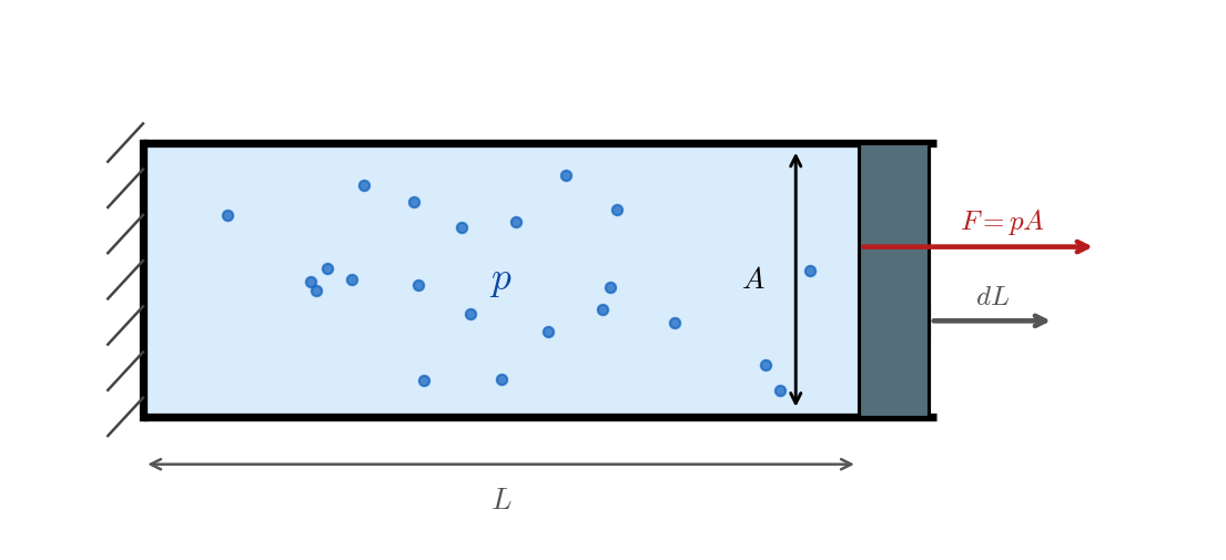
Example 1. Consider a gas with pressure \(p\), enclosed in a cylinder by a piston of area \(A\). The gas exerts a force \(F = pA\) on the piston. If the piston moves outward by an infinitesimal displacement \(dL\) (in m), the work done by the gas on the piston is \[ \delta W = pA \, dL = p \, dV, \tag{2.1}\] where \(dV = A \, dL\) is the infinitesimal increase in volume. We write \(\delta W\) rather than \(dW\) to signal that \(W\) is not a state function and the infinitesimal work is not an exact differential; the distinction between exact and inexact differentials will be made precise below.
Here \(p\) is the pressure the gas exerts at the moving boundary. For a quasi-static process the gas is uniform and this equals its thermodynamic pressure; it coincides with the external pressure as well only for an ideal, frictionless piston in mechanical equilibrium, that is, in the reversible case. If the piston is moved rapidly the gas is no longer uniform, its boundary pressure is not the equilibrium \(p\), and the work is governed instead by the external pressure. We return to this point in Lecture 7.
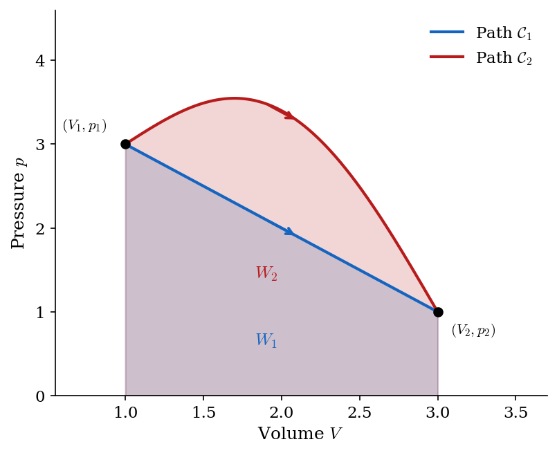
For a finite quasi-static process, the system traces a curve \(\mathcal{C}\) in the \((V,p)\) plane from state 1 to state 2. If the curve \(\mathcal{C}\) can be represented as a function \(V \mapsto p(V)\), then the work done by the gas along the curve is given by the integral: \[ W = \int_{V_1}^{V_2} p(V)\, dV. \tag{2.2}\] Geometrically, the work done by the gas is the area under the curve \(\mathcal{C}\) in the \((V,p)\) plane with a plus sign if the curve is traversed from left to right (expansion) and a minus sign if it is traversed from right to left (compression), as represented in Figure 2.2. Since different curves connecting the same initial and final states can have different areas under them, the work depends on the path taken from state 1 to state 2, not just on the endpoints. This is a crucial point: work is not a state function.
More generally, if we parametrize the curve \(\mathcal{C}\) by any parameter \(t \in [t_1, t_2]\) such that \((p(t), V(t))\) traces the process from state 1 to state 2, then \[ W = \int_{t_1}^{t_2} p(t)\, \dot{V}(t)\, dt, \tag{2.3}\] where \(\dot{V}(t) = dV/dt\). For instance, one may take \(t\) to be the time, but it could be any other parameter that monotonically increases along the curve. The value of the integral does not depend on the choice of parameterization, as long as it traces the same curve \(\mathcal{C}\).
Example 2. Consider a paramagnetic gas (molecular oxygen \(\mathrm{O_2}\) is a natural example) subject to a uniform external magnetic field \(B\) in a given fixed direction. The gas develops a magnetization \(M\) (defined as the total magnetic dipole moment per unit volume) in the same direction as \(B\). When the magnetic field changes by an infinitesimal amount \(dB\), the work done by the gas on the external field is given by \[ \delta W = -\alpha(N/V) \, V \, M \,dB. \tag{2.4}\] where, in general, \(\alpha(N/V)\) is a dimensionless constant that depends on the type of material and its density and it goes to one in the limit of low density. For a finite quasi-static process along a curve \(\mathcal{C}\) in the \(M\)–\(B\) plane: \[ W = - \int_{\mathcal{C}} \alpha(N/V) \, V \, M \,dB. \] As in Example 1, the integral depends on the path \(\mathcal{C}\), not only on the endpoints: magnetic work is not a state function. Since \(\mathrm{O_2}\) is also compressible, both types of work are active simultaneously, and the total work done by the gas in a quasi-static process and in the limit of low density is the sum of the two contributions: \[ \delta W = p\,dV - V M \,dB. \tag{2.5}\]
2.2.2 Thermal equilibrium and adiabatic walls
Consider two systems, each separately in thermodynamic equilibrium. Enclose them in containers that do not permit the exchange of matter and put the two containers in contact. Constrain the arrangement so that no work is exchanged between the two systems or between either system and the surroundings.
For a gas or liquid, this is achieved by making sure that the containers are rigid so that they cannot be compressed or expanded. In this case, the volumes are fixed and no \(p\,dV\) work can be exchanged. For magnetic substances it is achieved by making sure that the containers shield each magnetic substance from the magnetic field of the other, so that the magnetic field felt by each substance does not change and no magnetic work can be exchanged. For a more general system, one would have to design the containers to prevent all possible forms of work exchange, but the principle is the same.
The combined system is, in general, not in equilibrium: the macroscopic properties of each subsystem begin to change, and in general the two subsystems are driven out of equilibrium. After a sufficient time, however, the combined system settles into a new state of thermodynamic equilibrium. When this happens, we say the two systems are in thermal equilibrium with one another.
Thermal equilibrium — a relation between two systems: they are in thermal equilibrium if, when placed in thermal contact, no further change occurs. Distinct from thermodynamic equilibrium, which is a property of a single system.
Notice that the concepts of thermodynamic equilibrium and thermal equilibrium are related but different. Thermodynamic equilibrium is a property of a system, while thermal equilibrium defines a relation between two systems which are separately in thermodynamic equilibrium. Two systems may be separately in thermodynamic equilibrium but not in thermal equilibrium with each other.
When the conditions that allow the two system to evolve towards mutual thermal equilibrium are satisfied, while neither matter nor work is exchanged, we say the two systems are in thermal contact.
The time needed for the two systems to reach thermal equilibrium is called the thermalization time or thermal relaxation time, and it depends on the nature of the container walls. In layman’s terms, walls with longer thermalization times are better insulators, while walls with shorter thermalization times are better conductors. It is a matter of experience that one can design walls with an arbitrarily long thermalization time. Walls with an infinite thermalization time are called adiabatic: they are an idealization, which can be approximated arbitrarily well by real walls.
Two systems in contact through adiabatic walls, and otherwise isolated, can each undergo arbitrary changes of state (including large changes in pressure and volume) without ever coming to mutual thermal equilibrium. A process carried out entirely within adiabatic walls, so that the system is at no point in thermal contact with any other body, is called an adiabatic process.
Adiabatic process — a process in which the system exchanges no heat with its surroundings (\(Q = 0\)).
2.2.3 Adiabatic work and internal energy
For an adiabatic process, experiment establishes a remarkable fact: the work required to bring a system from a given initial state to a given final state is independent of the manner in which the adiabatic process is carried out. It depends only on the initial and final states.
This experimental observation is of fundamental importance. It is not obvious: whether a piston is pushed slowly or rapidly, if the process is adiabatic and brings the system from the same state \(A\) to the same state \(B\), the work required is exactly the same.
This dependence on the initial and final states alone permits us to define a function of state. We fix some arbitrarily chosen reference state \(O\), to which we assign zero energy by convention. Given a state \(A\), if an adiabatic process exists that takes the system from the state \(O\) to the state \(A\), we define the internal energy \(U(A)\) of the state \(A\) by \[ U(A) = -W_{\rm ad}(O \to A). \tag{2.6}\] If an adiabatic process exists that takes the system from the state \(A\) to the state \(O\), we define the internal energy \(U(A)\) of the state \(A\) by \[ U(A) = W_{\rm ad}(A \to O). \tag{2.7}\] In both cases, \(W_{\rm ad}\) is the work done by the system in the adiabatic process.
Internal energy \(U\) — a state function defined by the path-independent work required to reach a state adiabatically from a reference state \(O\).
C 2.1 The internal energy is well defined by Equation 2.6 and Equation 2.7 as a function of state.
Proof – Since the reference state \(O\) is fixed once and for all, the adiabatic work in Equation 2.6 depends only on the state \(A\) and not on the process itself: if two adiabatic processes exist that take the system from \(O\) to \(A\), the internal energy defined by Equation 2.6 does not depend on the process, but only on the state \(A\). The same argument can be used for the internal energy defined by Equation 2.7. It also needs to be noticed that, for the two definitions to be compatible, if adiabatic processes exist in both directions, Equation 2.6 and Equation 2.7 should give the same value for the internal energy. This happens if and only if \(W_{\rm ad}(O \to A) = - W_{\rm ad}(A \to O)\). Let us prove this compatibility equation.
If adiabatic processes exist in both directions, one can consider a composite process \(O \to A \to O\) obtained by executing the adiabatic process from \(O\) to \(A\) first and the adiabatic process from \(A\) to \(O\) after. The work done by the system through the composite process is equal to the sum of the works done through each individual process. Moreover, the composite process is adiabatic as well (since the whole composite process happens inside adiabatic walls). Therefore, the adiabatic work done through the composite process \(O \to A \to O\) depends only on the initial and final state and it is equal to the adiabatic work done through the trivial process, i.e. the process in which nothing is done to the system. This work is therefore zero, yielding \[ W_{\rm ad}(O \to A) + W_{\rm ad}(A \to O) = W_{\rm ad}(O \to A \to O) = W_{\rm ad}(O \to O) = 0. \tag{2.8}\] This equation is indeed the desired compatibility condition.
Summarizing, at fixed reference state \(O\), Equation 2.6 and Equation 2.7 define the internal energy as a function of the state \(A\).
C 2.2 Given an adiabatic process from \(A\) to \(B\), the following formula holds: \[ U(B) - U(A) = -W_{\rm ad}(A \to B) , \tag{2.9}\] i.e. the energy difference \(\Delta U = U(B) - U(A)\) is equal to the work done on the system through the adiabatic process from \(A\) to \(B\).
Proof – In order to prove this statement, we need to consider the following four cases separately:
- adiabatic processes \(O \to A\) and \(O \to B\) exist;
- adiabatic processes \(O \to A\) and \(B \to O\) exist;
- adiabatic processes \(A \to O\) and \(O \to B\) exist;
- adiabatic processes \(A \to O\) and \(B \to O\) exist.
We consider only case 1, the other ones can be treated analogously and are left to the students.
Consider the composite process \(O \to A \to B\). Since this process is also adiabatic, the energy of \(B\) is given by \(U(B) = -W_{\rm ad}(O \to A \to B)\) (see Equation 2.6). The work of the composite process is the sum of the works over the individual processes, one has \(U(B) = -W_{\rm ad}(O \to A) -W_{\rm ad}(A \to B) = U(A) -W_{\rm ad}(A \to B)\), where we have used Equation 2.6 again. Solving for \(U(B) - U(A)\), one obtains the desired result.
Of course, the definition of the energy depends also on the choice of reference state \(O\). Changing the state \(O\) amounts to shifting the energy by an overall constant (Problem 2.1). This is of no consequence: it is always true that energies are defined up to arbitrary additive constants. The energy itself is not a true physical observable, only energy differences are, and these are independent of the reference state as shown by Equation 2.9.
It is worth noticing that the definition of internal energy given here works only for states that are adiabatically connected to the reference state, i.e. states \(A\) for which an adiabatic process exists either from \(O\) to \(A\), or from \(A\) to \(O\). We will assume that any state is, in fact, adiabatically connected to any other and, therefore, the internal energy is defined for any state. This delicate point is usually not addressed in standard textbooks and I am not aware of any thermodynamic system that violates it. We will see later on how this works in the case of an ideal gas.
2.2.4 First Law and definition of heat
Equation 2.9 shows that, for an adiabatic process \(\Delta U = - W\), where \(\Delta U\) is the energy difference between final and initial state, while \(W\) is the work done by the system during the process.
Consider now a non-adiabatic process. Energy is conserved, so the change \(\Delta U\) in energy must be fully accounted for by energy exchanged across the boundary. Work accounts for part of it, but in general \(W \neq -\Delta U\). For closed systems, the remaining energy transfer, the part that is not work, we call heat and denote \(Q\). By this definition, \[ Q = \Delta U + W. \tag{2.10}\] Like work, heat is not a state function: its value depends on the path. We can now state the result compactly.
Heat \(Q\) — energy transferred across a boundary by any means other than work. Not a state function; depends on the path.
P 2.1 (First Law of Thermodynamics) For any closed system in thermodynamic equilibrium, there exists a state function \(U\), the internal energy, such that for any process taking the system from state \(A\) to state \(B\): \[ \Delta U = Q - W, \tag{2.11}\] where \(\Delta U = U(B) - U(A)\) is the variation of internal energy, \(Q\) is the heat absorbed by the system and \(W\) is the work done by the system.
The generalization of the First Law to open systems, in which matter crosses the boundary and the number of particles is no longer fixed, requires additional terms involving the chemical potential and will be discussed in a later lecture. For an infinitesimal process: \[ dU = \delta Q - \delta W. \tag{2.12}\] We write \(\delta Q\) and \(\delta W\) with the symbol \(\delta\) rather than \(d\) to indicate that these are inexact differentials, infinitesimal quantities that are not the differentials of any state function. The combination \(\delta Q - \delta W\), however, is exact: it equals \(dU\). This distinction is not merely notational. \(Q\) and \(W\) separately depend on the path; their difference does not.
Inexact differential \(\delta f\) — an infinitesimal quantity that is not the differential of any function. \(\delta Q\) and \(\delta W\) depend on the path; \(dU = \delta Q - \delta W\) does not.
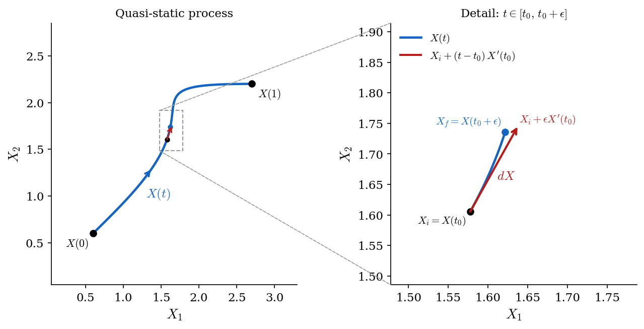
The equilibrium states of a generic thermodynamic system are identified by a set of independent variables \(X_1, \dots, X_n\) which we can pack into a vector \(X = (X_1, \dots, X_n)\). For instance, for a gas \(X = (V,p)\). A quasi-static process is a curve in the space of states, which can be generically parametrized as \(X(t)\) where one can always choose the parameter \(t\) to vary in the interval \([0,1]\). \(X(0)\) and \(X(1)\) are the initial and final states of the process, respectively.
Instead of looking at the whole process, we will look at the portion corresponding to \(t \in [t_0,t_0+\epsilon]\), where \(\epsilon\) is positive and infinitesimally small. Mathematically this means that we are going to consider the \(\epsilon \to 0^+\) limit. In this limit, assuming smoothness, the curve in the space of states can be approximated by a straight line (i.e. the tangent line) as shown by Taylor expanding \(X(t)\): \[ X(t) \overset{\epsilon \to 0^+}{=} X(t_0) + (t-t_0) X'(t_0) + O(\epsilon^2) , \quad \text{for } t \in [t_0,t_0+\epsilon] . \] The initial and final states for the infinitesimal process corresponding to \(t \in [t_0,t_0+\epsilon]\) are \[ X_i = X(t_0) , \quad X_f = X(t_0+\epsilon) \overset{\epsilon \to 0^+}{=} X_i + \epsilon X'(t_0) + O(\epsilon^2) . \] One can think of the exact differential \(dX\) as the difference between final and initial state up to \(O(\epsilon^2)\) corrections: \[ dX \overset{\text{def.}}{=} \epsilon X'(t_0) , \] which allows to write, in a suggestive notation: \[ X_f \overset{\epsilon \to 0^+}{=} X_i + dX + O(\epsilon^2) . \]
The energy of the final state can be expanded in powers of \(\epsilon\) as well: \[ U(X_f) \overset{\epsilon \to 0^+}{=} U(X_i) + \epsilon \nabla U(X_i) \cdot X'(t_0) + O(\epsilon^2) \] \[ = U(X_i) + \nabla U(X_i) \cdot dX + O(\epsilon^2) . \] One can think of the exact differential \(dU\) as the difference between final and initial energy up to \(O(\epsilon^2)\) corrections: \[ dU \overset{\text{def.}}{=} \nabla U(X_i) \cdot dX , \] which allows to write, in a suggestive notation: \[ \Delta U(\epsilon) = U(X_f) - U(X_i) \overset{\epsilon \to 0^+}{=} dU + O(\epsilon^2) . \]
One can define the heat \(Q(\epsilon)\) absorbed by the system in the interval \(t \in [t_0,t_0+\epsilon]\) and, similarly, the work \(W(\epsilon)\) done by the system in the same interval. Notice that, if \(\epsilon=0\), then nothing is done to the system, initial and final state coincide and no heat and work are exchanged i.e. \(Q(0)=W(0)=0\). If \(\epsilon\) is positive but small, by Taylor expanding \(Q(\epsilon)\) and \(W(\epsilon)\) in powers of \(\epsilon\) one can write \[ Q(\epsilon) \overset{\epsilon \to 0^+}{=} \epsilon \dot{Q}(0) + O(\epsilon^2) , \quad W(\epsilon) \overset{\epsilon \to 0^+}{=} \epsilon \dot{W}(0) + O(\epsilon^2) . \] One can think of the inexact differentials \(\delta Q\) and \(\delta W\) as the heat absorbed by and the work done by the system in the infinitesimal process corresponding to \(t \in [0,\epsilon]\) up to \(O(\epsilon^2)\) corrections: \[ \delta Q \overset{\text{def.}}{=} \epsilon \dot{Q}(0) , \quad \delta W \overset{\text{def.}}{=} \epsilon \dot{W}(0) , \] which allows to write, in a suggestive notation: \[ Q(\epsilon) \overset{\epsilon \to 0^+}{=} \delta Q + O(\epsilon^2) , \quad W(\epsilon) \overset{\epsilon \to 0^+}{=} \delta W + O(\epsilon^2) . \]
The first law of thermodynamics, which holds for any process, can be written as \[ \Delta U(\epsilon) \overset{\epsilon \to 0^+}{=} Q(\epsilon) - W(\epsilon) . \] Since this equation holds for any \(\epsilon\), then it has to hold also order by order in \(\epsilon\). In particular, at first order in \(\epsilon\) one obtains simply \[ dU = \delta Q - \delta W. \]
In general, \(dU\), \(\delta Q\) and \(\delta W\) will be linear scalar functions of \(d X\), i.e. \[ dU = f_U(X_i) \cdot dX , \quad \delta Q = f_Q(X_i) \cdot dX , \quad \delta W = f_W(X_i) \cdot dX , \] where \(f_U(X)\), \(f_Q(X)\) and \(f_W(X)\) are vector functions of the state variables \(X\). In fact, the definition of \(dU\) yields the explicit expression \(f_U(X) = \nabla U(X)\). The statement that \(dU\) is an exact differential is exactly the statement that \(f_U(X)\) is the gradient of a scalar function, while the statement that \(\delta Q\) and \(\delta W\) are inexact differentials is exactly the statement that \(f_Q(X)\) and \(f_W(X)\) are not gradients of any scalar function. As for conservative and non-conservative forces, the line integral of \(f_U(X)\) will depend only on initial and final states but not on the path connecting the two, while the line integral of \(f_Q(X)\) and \(f_W(X)\) will depend on the path.
The more mathematically minded can understand \(dU\), \(\delta Q\) and \(\delta W\) as differential one-forms: \(dU\) is a an exact form, while \(\delta Q\) and \(\delta W\) are inexact forms.
The First Law encodes two logically distinct facts: that a state function \(U\) exists (a consequence of the path-independence of adiabatic work) and that in any process \(\Delta U = Q - W\), which simultaneously serves as the definition of heat.
2.2.5 Remarks on the First Law
The First Law is a statement of energy conservation. The internal energy of an isolated system (\(Q = 0\), \(W = 0\)) is constant. Energy of a closed system may be transferred to or from the system as heat or as work, but the total is conserved.
Adiabatic walls prevent the exchange of heat, so any change in internal energy must be accounted for by work. If two systems, that are prevented from exchanging work, reach thermal equilibrium, they do so by exchanging heat.
The sign convention adopted here (\(Q > 0\) when heat flows into the system, \(W > 0\) when work is done by the system) gives \(\Delta U = Q - W\). An alternative convention, common in engineering and in some chemistry texts, takes \(W > 0\) when work is done on the system, which changes the First Law to \(\Delta U = Q + W\). The two conventions are entirely equivalent; care is needed when comparing results from different sources.
Neither heat nor work is a form of energy stored in a system. The system possesses internal energy \(U\); it does not possess “heat” or “work”. Heat and work are names for the two modes by which energy crosses the boundary: thermal transfer and mechanical transfer, respectively. They exist only in transit. Saying that a body “contains heat” is as meaningless, physically, as saying that a body “contains work”. The distinction is linguistically awkward but physically essential.
2.3 Summary
Systems and states
- A thermodynamic system is a portion of matter separated from its surroundings by a boundary. A closed system exchanges no matter; an isolated system exchanges neither matter nor energy.
- A system left undisturbed reaches thermodynamic equilibrium, a state fully specified by a small number of state variables. State variables are either extensive (proportional to system size) or intensive (independent of size).
Processes
- A quasi-static process is an idealised continuous succession of equilibrium states.
- Two systems placed in thermal contact (no work or matter exchanged) eventually reach mutual thermal equilibrium. Walls that prevent heat exchange are called adiabatic; a process within adiabatic walls is an adiabatic process.
Energy
- The work done by a system in a quasi-static process is \(W = \int_{\mathcal{C}} p\,dV\) for a fluid and \(W = -V\int_{\mathcal{C}} M\,dB\) for a magnetic substance. Work is path-dependent; it is not a state function.
- The work required to take a system between two states adiabatically is path-independent. This permits the definition of a state function, the internal energy \(U\).
- The First Law of Thermodynamics: for any process, \(\Delta U = Q - W\), where \(Q\) is the heat absorbed by the system and \(W\) is the work done by the system. Heat, like work, is path-dependent and is not a state function. Neither heat nor work is energy stored in the system; they are the two modes by which energy crosses the boundary.
| Quantity | Symbol | SI unit |
|---|---|---|
| Pressure | \(p\) | Pa \(=\) N m\(^{-2}\) \(=\) kg m\(^{-1}\) s\(^{-2}\) |
| Volume | \(V\) | m\(^3\) |
| Temperature | \(T\) | K |
| Amount of substance | \(n\) | mol |
| Number of molecules | \(N\) | (dimensionless) |
| Magnetic field | \(B\) | T \(=\) kg A\(^{-1}\) s\(^{-2}\) |
| Magnetization (dipole moment per unit volume) | \(M\) | A m\(^{-1}\) |
| Work | \(W\) | J \(=\) kg m\(^2\) s\(^{-2}\) |
| Internal energy | \(U\) | J |
| Heat | \(Q\) | J |
| Constant | Symbol | SI unit | Value |
|---|---|---|---|
| Avogadro constant | \(N_A\) | mol\(^{-1}\) | \(6.022 \times 10^{23}\) mol\(^{-1}\) |
| Boltzmann constant | \(k_B\) | J K\(^{-1}\) | \(1.381 \times 10^{-23}\) J K\(^{-1}\) |
2.4 Problems
Problem 2.1 Two choices of reference state \(O\) and \(O'\) are used to define internal energies \(U\) and \(U'\) by means of Equation 2.6. Show that \(U'(A) = U(A) + k\) where \(k\) is a constant that does not depend on the state \(A\).
Problem 2.2 A gas is taken quasi-statically from state \((p_0, V_0)\) to state \((2p_0, 2V_0)\) by two paths: along path I, the gas first expands isobarically (at constant pressure) to \((p_0, 2V_0)\), then its pressure is raised isochorically (at constant volume) to \((2p_0, 2V_0)\); along path II, the pressure is first raised isochorically to \((2p_0, V_0)\), then the gas expands isobarically to \((2p_0, 2V_0)\). Compute the work done by the gas along each path.
Problem 2.3 An ideal gas (\(pV = nRT\)) expands quasi-statically and isothermally (at constant temperature \(T\), with \(n\) fixed) from volume \(V_1\) to \(V_2 > V_1\). Compute the work done by the gas.
Problem 2.4 A system is taken from state \(A\) to state \(B\) along path \(\mathcal{C}_1\), absorbing heat \(Q_1 = 120\ \mathrm{J}\) and doing work \(W_1 = 50\ \mathrm{J}\). It is then returned from \(B\) to \(A\) along path \(\mathcal{C}_2\), during which it does work \(W_2 = -20\ \mathrm{J}\). (a) Find the heat \(Q_2\) absorbed along \(\mathcal{C}_2\). (b) Find the net heat absorbed and net work done in the complete cycle.
Problem 2.5 Show that the net work done by a gas in a quasi-static cyclic process equals the area enclosed by the cycle in the \((V,p)\) plane, with a positive sign if the cycle is traversed clockwise and a negative sign if traversed counterclockwise.
Problem 2.6 A paramagnetic gas (in the low-density limit, \(\alpha = 1\)) is taken quasi-statically from state \((M_0, B_0)\) to state \((2M_0, 2B_0)\) by two paths in the \(M\)–\(B\) plane. Along path I, the magnetization is first doubled at constant field to \((2M_0, B_0)\), then the field is doubled at constant magnetization to \((2M_0, 2B_0)\). Along path II, the field is first doubled at constant magnetization to \((M_0, 2B_0)\), then the magnetization is doubled at constant field. Using \(\delta W = -V M\, dB\), compute the work done by the gas along each path. Does the work depend on the path?
Problem 2.7 A gas is enclosed in an adiabatic container. In experiment 1, a piston compresses the gas quasi-statically from state \(A\) to state \(B\), with \(200\ \mathrm{J}\) of work done on the gas. In experiment 2, the same change of state is achieved by a rapidly moving piston, with \(230\ \mathrm{J}\) of work done on the gas. Are these results consistent with the path-independence of adiabatic work? What can be concluded about \(U(B) - U(A)\) in each case?
Problem 2.8 A gas occupies half of a rigid thermally insulated container of total volume \(2V_0\), separated from the evacuated other half by a partition. The partition is suddenly removed and the gas expands to fill the whole container.
What work does the gas do during the expansion? What is \(\Delta U\)?
Mark the initial state \((p_0, V_0)\) and the final state \((p_1, 2V_0)\) as points in the \((V,p)\) plane. Can the process be represented as a curve connecting them? Why not?
A quasi-static isothermal expansion of an ideal gas from \(V_0\) to \(2V_0\) can be drawn as a curve in the \((V,p)\) plane. What work does the gas do in that case? Compare the two processes: they share the same initial and final volumes, but are they the same process?
Problem 2.9 Two systems have the following equations of state. An ideal gas satisfies \(pV = nRT\), where \(n\) is the number of moles and \(R\) is the gas constant. A photon gas (electromagnetic radiation in thermal equilibrium inside a cavity) satisfies \(p = \tfrac{1}{3}aT^4\), where \(a = 8\pi^5 k_B^4 / (15 h^3 c^3) \simeq 7.57 \times 10^{-16}\ \mathrm{J\,m^{-3}\,K^{-4}}\) is the radiation constant.
Sketch the isothermal curves (\(T = \mathrm{const}\)) in the \((V,p)\) plane for the ideal gas at two temperatures \(T_1 < T_2\). What is the shape of each curve?
Sketch the isothermal curves in the \((V,p)\) plane for the photon gas at the same two temperatures. What is qualitatively different compared to the ideal gas?
Problem 2.10 A monoatomic ideal gas has equation of state \(pV = nRT\) (with \(n\) fixed) and internal energy \(U = \tfrac{3}{2}pV\). The gas is taken quasi-statically from state \(A = (p_0, V_0)\) to state \(B = (2p_0, 2V_0)\) along two paths in the \((V,p)\) plane:
- Path I: isobaric expansion from \(A\) to \((p_0, 2V_0)\), then isochoric pressure increase to \(B\).
- Path II: isochoric pressure increase from \(A\) to \((2p_0, V_0)\), then isobaric expansion to \(B\).
For each path compute \(W\), \(\Delta U\) and \(Q\). Which quantities depend on the path?
Problem 2.11 A photon gas has equation of state \(p = \tfrac{1}{3}aT^4\) and internal energy \(U = 3pV\). The gas is taken quasi-statically from state \(A = (p_0, V_0)\) to state \(B = (2p_0, 2V_0)\) along the same two paths as in Problem 2.10.
For each path compute \(W\), \(\Delta U\) and \(Q\). Note that for the photon gas, pressure depends on temperature alone; what does this imply for path I?
Problem 2.12 A differential form \(f_1(V,p)\,dV + f_2(V,p)\,dp\) is exact if and only if \[ \frac{\partial f_1}{\partial p} = \frac{\partial f_2}{\partial V} . \] This is the integrability condition: it tests whether \(f = (f_1 , f_2)\) is the gradient of some scalar function.
Consider a monoatomic ideal gas with state space \((V, p)\), equation of state \(pV = nRT\) (with \(n\) fixed), internal energy \(U = \tfrac{3}{2}pV\), and \(\delta W = p\,dV\).
Write \(dU\) explicitly as a linear form \(f_1\,dV + f_2\,dp\) and verify that it satisfies the integrability condition. Verify also that \(f_1\) and \(f_2\) are the partial derivatives of \(U\).
Write \(\delta W\) as a linear form and check the integrability condition.
Use the First Law \(\delta Q = dU + \delta W\) to derive \(\delta Q\) as a linear form, and check the integrability condition.
What do you conclude about \(dU\), \(\delta W\) and \(\delta Q\)?