4 Ideal Gases
Part I — Foundations
Last updated: 17-05-2026
The ideal gas is an idealization which can be approached arbitrarily closely by real gases in the limit of low density.
4.1 Equation of state
One of the most important properties of gases in the low-density limit is that their equation of state becomes independent of the composition of the gas and takes the simple form \[ pV = N k_B T, \tag{4.1}\] where \(N\) is the number of molecules, \(T\) is the temperature as defined in Section 3.3.2, \(p\) is the pressure and \(V\) is the volume. The universal constant \(k_B\) is called the Boltzmann constant and has the value \(k_B \approx 1.38 \times 10^{-23}\ \mathrm{J\ K^{-1}}\). By introducing the number of moles \(n = N/N_A\), the equation of state of the ideal gas can also be written equivalently as \[ pV = n R T, \tag{4.2}\] with the definition \(R = N_A k_B = 8.314\ \mathrm{J\ mol^{-1}\ K^{-1}}\).
Let us see that the equation of state is compatible with the definition of ideal gas temperature given in Equation 3.3. When the ideal gas thermometer is in thermal equilibrium with water at its triple point, the gas has temperature \(T_\mathrm{tr} = 273.16\ \mathrm{K}\) and pressure \(p_\mathrm{tr} = N k_B T_\mathrm{tr} / V\). At a generic temperature \(T\), the ideal gas thermometer has pressure \(p = N k_B T/ V\) (notice that \(N\) and \(V\) are fixed in the thermometer). Therefore \[ \frac{p}{p_\mathrm{tr}} = \frac{T}{T_\mathrm{tr}} , \tag{4.3}\] which is indeed equivalent to Equation 3.3.
4.2 Internal energy
Unlike the equation of state, the internal energy of an ideal gas depends on the composition of the gas and is not universal. Experimentally one observes that, at fixed number of molecules \(N\) or (which is the same) moles \(n\), in the limit of low density the internal energy of a gas depends on the temperature but not on the volume.
This fact can be established by studying the free expansion of a gas into vacuum, as first done by Joule in 1845. A gas is confined in one compartment of a thermally insulated rigid vessel, with the adjacent compartment evacuated. When the connection between the two compartments is opened, the gas expands into vacuum. Since the gas does no work (\(W = 0\)) and no heat is exchanged (\(Q = 0\)), the First Law requires \(\Delta U = 0\): the internal energy is unchanged. If the density of the gas is low enough, one observes that the temperature after the free expansion is the same as before. This means that, by changing \(V\) at fixed \(T\) and \(n\), the internal energy does not change.
We conclude that the internal energy is a function of \(n\) and \(T\). Since it is an extensive quantity, it must be proportional to \(n\), yielding \[ U = n\, u(T), \tag{4.4}\] where \(u\) is the molar internal energy (internal energy per mole).
Molar heat capacity and the energy. Differentiating Equation 4.4 at constant \(V\) and \(n\): \[ C_V = \left(\frac{\partial U}{\partial T}\right)_{V,n} = n\,\frac{du}{dT} \equiv n\,c_V(T), \] where \(c_V(T) = du/dT\) (in J mol\(^{-1}\) K\(^{-1}\)) depends only on temperature. Inverting: \[ dU = n\,c_V(T)\,dT = C_V\,dT. \tag{4.5}\] This holds for any process of an ideal gas, not only constant-volume ones, since \(U\) depends only on \(T\). Integrating between a reference temperature \(T_0\) and \(T\): \[ U(T) - U(T_0) = n\int_{T_0}^{T} c_V(T')\,dT'. \tag{4.6}\] Only differences of \(U\) are physically meaningful; the choice of \(T_0\) is a convention (cf. the discussion of reference states in Section 2.2.3).
Values of \(c_V\). The molar heat capacity must be determined experimentally; its value reflects the molecular structure of the gas. This is in sharp contrast to the equation of state \(pV = nRT\), which is universal: all dilute gases obey it regardless of their composition, and it makes no distinction between helium, hydrogen, or chlorine. The energy function \(u(T)\), characterized by \(c_V(T)\), is substance-specific: it encodes information about molecular structure that the equation of state does not contain. A complete thermodynamic description of an ideal gas therefore requires two inputs — the mechanical equation of state and the caloric equation of state \(c_V(T)\) — and the second must be measured separately for each substance.
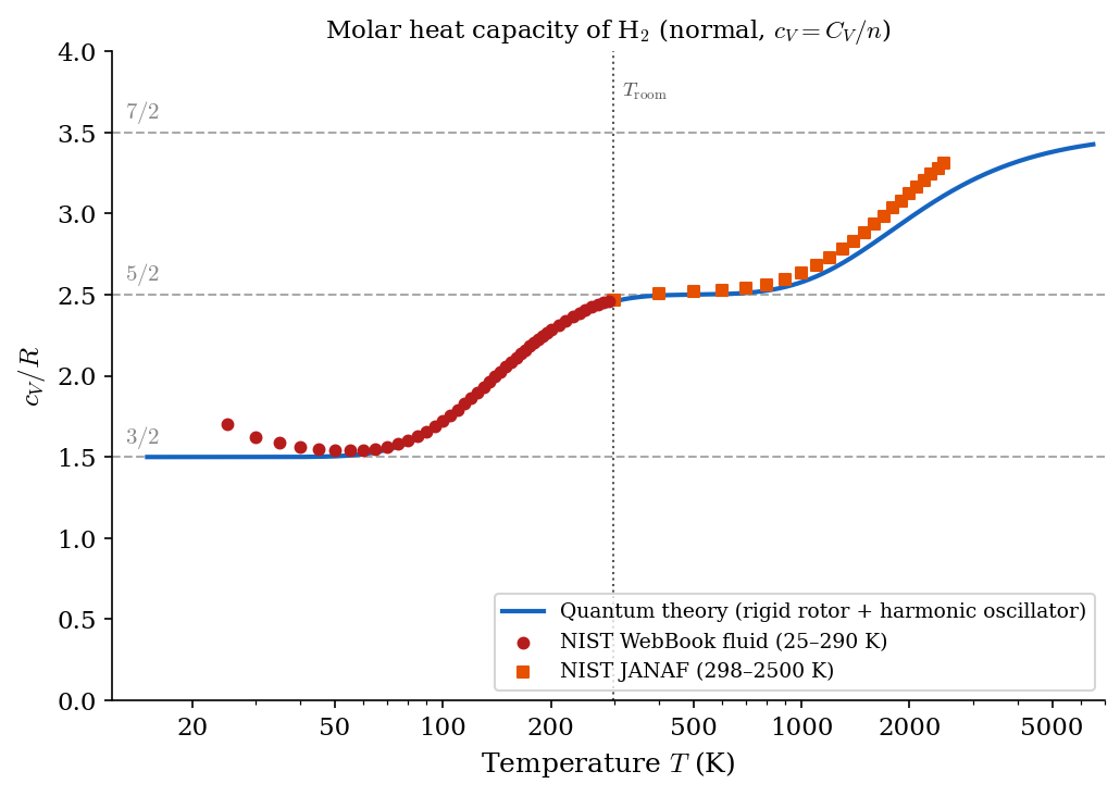
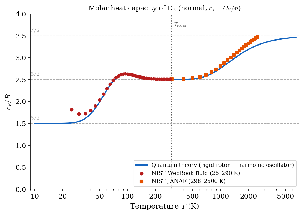
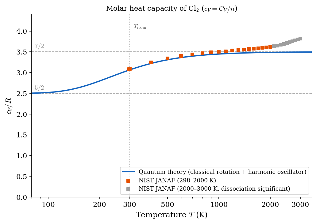
In general, for ideal gases one finds that \(c_V(T)\) is positive and a non-decreasing function of the temperature. All monatomic ideal gases (e.g., He, Ar, Ne) have \(c_V \approx \frac{3}{2}R\) in a large range of temperatures (which includes room temperature). Many diatomic gases have \(c_V \approx \frac{5}{2}R\) close to room temperature. However, when a large range of temperature is explored, one sees a richer structure, which is illustrated by a mix of theoretical predictions and semi-empirical data in Figure 4.1, Figure 4.2 and Figure 4.3 for H\(_2\), D\(_2\), and Cl\(_2\) respectively.
As you will learn from Statistical Mechanics, the temperature dependence of \(c_V\) is a purely quantum phenomenon with no classical explanation. In fact, any classical model of the ideal gas, yields a constant \(c_V\). If atoms are idealized as point-like particles, Classical Statistical Mechanics, for a diatomic gas, gives \(c_V = \frac{7}{2}R\) regardless of \(T\) in flat contradiction with the figures below. On the other hand, Quantum Statistical Mechanics yields the typical staircase structure of \(c_V(T)\), with plateaus at \(\frac{3}{2}R\), \(\frac{5}{2}R\), and \(\frac{7}{2}R\) which is much more in agreement with the semi-empirical data. One usually thinks that quantum effects become visible only at the microscopic scale. However, the figures below show that quantum effects can be visible at macroscopic scales as well: in this case, in the form of a non-trivial temperature dependence of \(c_V\).
4.3 Adiabatic index
Dividing Equation 3.8 by \(n\), we obtain the relation \[ c_p = \left( \frac{\partial u}{\partial T} \right)_p + \frac{p}{n} \left( \frac{\partial V}{\partial T} \right)_p. \tag{4.7}\] The first partial derivative is calculated using the fact that \(u\) depends only on \(T\) (therefore neither on the pressure nor on the volume), which yields \[ \left( \frac{\partial u}{\partial T} \right)_p = \frac{du}{dT} = \left( \frac{\partial u}{\partial T} \right)_V = c_v(T) . \tag{4.8}\] The second partial derivative is calculated using the equation of state, i.e. \[ \left( \frac{\partial V}{\partial T} \right)_p = \left( \frac{\partial}{\partial T} \frac{n R T}{p} \right)_p = \frac{n R}{p} . \tag{4.9}\] Combining the above three equations we obtain the molar heat capacity at constant pressure: \[ c_p(T) = c_V(T) + R . \tag{4.10}\]
Mayer’s relation — \(c_p = c_V + R\) for any ideal gas. The extra \(R\) accounts for the work done in expanding against constant pressure.
For the ideal gas, both molar heat capacities depend only on temperature. The adiabatic index is then given by \[ \gamma(T) = \frac{c_p(T)}{c_V(T)} = 1 + \frac{R}{c_V(T)}. \tag{4.11}\] Since \(c_V\) is positive, the adiabatic index is larger than one.
For temperatures close to room temperature, one can often use the following approximation for monatomic ideal gases: \[ c_V \approx \frac{3}{2}R, \quad c_p \approx \frac{5}{2}R, \quad \gamma \approx \frac{5}{3}, \tag{4.12}\] and the following rough approximation for diatomic gases: \[ c_V \approx \frac{5}{2}R, \quad c_p \approx \frac{7}{2}R, \quad \gamma \approx \frac{7}{5}. \tag{4.13}\]
4.4 Isothermal process
In the \((V,p)\) plane, isothermal curves are defined as the curves along which the temperature is constant. Since \(pV = nRT\), the isothermal curve corresponding to temperature \(T\) is described by the equation \[ p(V) = \frac{nRT}{V} . \tag{4.14}\] Different values of \(T\) yield different isothermal curves.
An isothermal process is a quasi-static process along which the temperature stays constant, while the volume changes slowly from \(V_1\) to \(V_2\) and the gas is an equilibrium state at every intermediate point. The work done by the gas in this process is given by \[ W = \int_{V_1}^{V_2} p \, dV = nRT \int_{V_1}^{V_2} \frac{dV}{V} = nRT \ln \frac{V_2}{V_1}. \tag{4.15}\] Since, for an ideal gas, the internal energy depends on the temperature but not on the volume, then the internal energy stays constant during the process and, in particular \(\Delta U = 0\). The First Law implies that the system absorbs heat \(Q = W\).
Isothermal process — a quasi-static process at constant temperature. For an ideal gas: \(\Delta U = 0\), \(Q = W = nRT\ln(V_2/V_1)\).
If \(V_2>V_1\), then the process is an isothermal expansion. In this case, since \(W = Q > 0\), the system absorbs heat from the environment and delivers work to the environment. If \(V_2 < V_1\), then the process is an isothermal compression. In this case, since \(W = Q < 0\), the system releases heat into the environment and extracts work from the environment.
4.5 Quasi-static adiabatic process
A quasi-static adiabatic process is one in which no heat is exchanged (\(Q = 0\)) and the process is quasi-static, so that the pressure is well-defined at every instant and the work is given by \(\delta W = p\,dV\). Applying the First Law to an infinitesimal step, \(dU = -\delta W = -p \, dV\), and substituting Equation 4.5:
Quasi-static adiabatic process — no heat exchange (\(Q = 0\)), pressure well-defined at every instant. For an ideal gas with constant \(\gamma\): \(TV^{\gamma-1} = \mathrm{const}\), \(pV^\gamma = \mathrm{const}\).
\[ n \, c_V \, dT = C_V \, dT = -p \, dV = -\frac{nRT}{V} dV. \tag{4.16}\] Separating variables and using the formula for the adiabatic index (Equation 4.11) \[ \frac{dV}{V} = - \frac{c_V(T)}{R} \, \frac{dT}{T} = \frac{1}{1 - \gamma(T)} \, \frac{dT}{T} \tag{4.17}\] Given an initial state with temperature \(T_0\) and volume \(V_0\), along a quasi-static adiabatic process the temperature \(T\) changes with the volume \(V\), i.e. the temperature is a function \(T = T(V)\). Integrating Equation 4.17 between the states \((V_0,T_0)\) and \((V,T(V))\) yields \[ \log \frac{V}{V_0} = \int_{T_0}^{T(V)} \frac{1}{1 - \gamma(\tau)} \, \frac{d\tau}{\tau} \ , \tag{4.18}\] which has to be seen as an equation for \(T(V)\).
An explicit solution for \(T(V)\) can be found only by modelling the temperature dependence of the adiabatic index. If the adiabatic index can be considered approximately constant in the range of temperatures considered, Equation 4.18 reduces to \[ \log \frac{V}{V_0} = \frac{1}{1 - \gamma} \, \log \frac{T(V)}{T_0} \ , \tag{4.19}\] which can also be rearranged as \[ T(V) = \left( \frac{V_0}{V} \right)^{\gamma-1} T_0 \tag{4.20}\] The value of the pressure along the process is given by \[ p(V) = \frac{nRT(V)}{V} = \left( \frac{V_0}{V} \right)^{\gamma} p_0 \ . \tag{4.21}\] The function \(p(V)\) determines the adiabatic curve in the \((p,V)\) plane passing through the state \((V_0,p_0)\). These curves are the trajectories of quasi-static adiabatic processes; a non-quasi-static adiabatic process (such as a free expansion) does not follow them, as explored in Problem 4.5.
Adiabatic curve — the trajectory \(pV^\gamma = \mathrm{const}\) in the \((p,V)\) plane traced by a quasi-static adiabatic process. Steeper than an isotherm at every point (since \(\gamma > 1\)).
Consider now a quasi-static adiabatic process starting from the state with temperature \(T_1\) and volume \(V_1\), and terminating when the volume reaches \(V_2\). Assuming a constant adiabatic index (which implies a constant molar heat capacity), the work done by the gas in this process is given by \[ W = - \Delta U = - n \int_{T_1}^{T_2} c_V \, dT = - n c_V (T_2 - T_1) = n c_V T_1 \left[ 1 - \left( \frac{V_1}{V_2} \right)^{\gamma-1} \right] . \tag{4.22}\] Recall that \(\gamma-1>0\). If \(V_2>V_1\), then the process is a quasi-static adiabatic expansion. In this case, \(W > 0\) and the system delivers work to the environment. If \(V_2 < V_1\), then the process is a quasi-static adiabatic compression. In this case, \(W < 0\) and the system extracts work from the environment.
4.6 Problems
Problem 4.1 Using Mayer’s relation Equation 4.10, compute \(c_p\) and \(\gamma\) for a monatomic ideal gas (\(c_V = \tfrac{3}{2}R\)) and for a diatomic ideal gas in the rotational plateau (\(c_V = \tfrac{5}{2}R\)) and in the vibrational plateau (\(c_V = \tfrac{7}{2}R\)). Show that \(\gamma > 1\) for any ideal gas, and that \(\gamma \to 1\) as \(c_V \to \infty\).
Problem 4.2 One mole of a monatomic ideal gas starts at temperature \(T_1 = 300\ \mathrm{K}\) and volume \(V_1 = 10\ \mathrm{L}\). It undergoes two successive quasi-static steps: (a) isothermal expansion to \(V_2 = 20\ \mathrm{L}\); (b) isochoric cooling to \(T_3 = 150\ \mathrm{K}\). For each step and for the overall process, compute \(\Delta U\), \(W\), and \(Q\).
Problem 4.3 A diatomic ideal gas (\(\gamma = 7/5\)) at temperature \(T_0\) and pressure \(p_0\) undergoes a quasi-static adiabatic expansion until its volume doubles. Find the final temperature and pressure, and compute the work done per mole. Compare with the work done in an isothermal expansion to the same final volume.
Problem 4.4 In the \((V,p)\) plane, the isotherm through a state \((p_0, V_0)\) satisfies \(pV = p_0 V_0\), and the quasi-static adiabat through the same state satisfies \(pV^\gamma = p_0 V_0^\gamma\).
Compute the slope \(dp/dV\) along the isotherm and along the adiabat at the point \((p_0, V_0)\). Express both in terms of \(p_0\), \(V_0\), and \(\gamma\).
Show that the adiabat is steeper than the isotherm at every point in the \((V,p)\) plane, and find the ratio of the two slopes.
Sketch both curves through the same point.
Problem 4.5 An ideal gas with adiabatic index \(\gamma\) is initially at temperature \(T_0\), pressure \(p_0\), and volume \(V_0\).
A quasi-static adiabatic expansion takes the gas from \(V_0\) to \(2V_0\). Find the final temperature \(T_1\) and verify that the final state lies on the curve \(pV^\gamma = p_0 V_0^\gamma\).
A free adiabatic expansion (into vacuum) takes the gas from \(V_0\) to \(2V_0\) instead. Find the final temperature \(T_2\) and pressure \(p_2\).
Compare \(T_1\) and \(T_2\). Show that the final state of the free expansion does not lie on the curve \(pV^\gamma = p_0 V_0^\gamma\), and identify the value of the constant \(C\) such that it lies on \(pV^\gamma = C\). What does this say about non-quasi-static adiabatic processes?
Problem 4.6 Starting from Equation 4.21, compute the work done by \(n\) moles of an ideal gas (with \(c_V\) constant) in a quasi-static adiabatic process from \((p_1, V_1)\) to \((p_2, V_2)\) by direct integration of \(\int_{V_1}^{V_2} p\,dV\). Show that the result can be written \[ W = \frac{p_1 V_1 - p_2 V_2}{\gamma - 1}, \] and verify that it agrees with Equation 4.22.
Problem 4.7 (More demanding.) Sound waves propagate through a gas via compressions and rarefactions that are quasi-static and adiabatic, not isothermal. The speed of sound is \(c_s = \sqrt{K_{\rm ad} / \rho_m}\), where \(\rho_m = nM/V\) is the mass density, \(M\) is the molar mass, and \(K_{\rm ad} = -V\,dp/dV\) is the adiabatic bulk modulus, with \(dp/dV\) taken along the adiabat through the current state. Using Equation 4.21, show that \(K_{\rm ad} = \gamma p\) and hence \[ c_s = \sqrt{\frac{\gamma RT}{M}}. \] Compute \(c_s\) for air (\(M \approx 29\ \mathrm{g\ mol^{-1}}\), \(\gamma = 7/5\)) at \(T = 293\ \mathrm{K}\) and compare with the measured value of \(343\ \mathrm{m\ s^{-1}}\).
Problem 4.8 (More demanding.) This problem establishes that any two states of an ideal gas are adiabatically connected in the sense of Section 2.2.3, using quasi-static adiabatic processes and free expansions. Assume \(\gamma\) is constant throughout.
Show that the quantity \(\sigma = TV^{\gamma-1}\) is constant along a quasi-static adiabatic process and strictly increases under a free expansion (in which \(V\) increases at constant \(T\)).
Let \(A = (T_A, V_A)\) and \(B = (T_B, V_B)\) be two states with \(\sigma_B \geq \sigma_A\), where \(\sigma_A = T_A V_A^{\gamma-1}\) and \(\sigma_B = T_B V_B^{\gamma-1}\). Show that \(B\) is reachable from \(A\) by a quasi-static adiabatic process followed by a free expansion. Identify the intermediate state \(C\) explicitly and verify that the free expansion step requires \(V_B \geq V_C\).
Hence show that any two states \(A\) and \(B\) are adiabatically connected: either \(B\) is reachable from \(A\), or \(A\) is reachable from \(B\) (or both, if \(\sigma_A = \sigma_B\)), by such a two-step process. Conclude that the internal energy \(U\) defined in Section 2.2.3 is well-defined for every state of an ideal gas.