9 Thermodynamic Potentials and Maxwell Relations
Part III — Potentials and Equilibrium
Last updated: 23-06-2026
9.1 Where this lecture is going
The last lecture closed with the fundamental relation in its open-system form, \[ dU = T\,dS - p\,dV + \mu\,dn, \tag{9.1}\] in which the temperature, pressure and chemical potential appear as the derivatives of the internal energy, \(T = (\partial U/\partial S)_{V,n}\), \(p = -(\partial U/\partial V)_{S,n}\) and \(\mu = (\partial U/\partial n)_{S,V}\) (Lecture 8). It is a differential relation, telling us how the energy changes between neighbouring equilibrium states. On it this lecture builds the standard machinery of thermodynamics: the finite relations that extensivity forces, the potentials suited to the variables an experimenter controls, and the identities those potentials yield.
Throughout, the system is a homogeneous body of a single substance, described by the variables \((S, V, n)\) with one chemical potential \(\mu\). A homogeneous system of several substances would carry one chemical potential per species, the term \(\mu\,dn\) becoming \(\sum_i \mu_i\,dn_i\); that extension is the subject of Lecture 11.
The first thread is extensivity, no new assumption but one we have used since the start. Pushed to its full conclusion it yields a finite relation among the state variables, the Euler relation, and from that the Gibbs–Duhem relation, which shows that the intensive variables \(T\), \(p\) and \(\mu\) are not independent; for a one-component substance \(\mu\) is a function of \(T\) and \(p\) alone.
The second thread is that the natural variables of the internal energy, \(S\) and \(V\), are not the ones an experiment usually fixes: the entropy, in particular, is almost never controlled directly, whereas the temperature is. A Legendre transform exchanges a natural variable for the intensive variable conjugate to it, producing three further potentials, the enthalpy, the Helmholtz free energy and the Gibbs free energy, each suited to a different pair of controlled variables. We then read what each potential measures physically, and finally extract from their mixed second derivatives the Maxwell relations, and from one of those the energy equation, which fixes the volume dependence of the internal energy through the equation of state.
This is the machinery lecture. The Gibbs free energy, the identity \(\mu = g\), the Gibbs–Duhem relation and the Maxwell and energy-equation identities assembled here are the working tools of the lectures on phase transitions (Lecture 10) and chemical equilibrium (Lecture 11) that follow.
9.2 Extensivity and the Euler relation
Extensivity is not a new assumption. We drew the distinction between extensive and intensive variables back in Lecture 2: an extensive variable, such as the volume \(V\), the amount of substance \(n\), the internal energy \(U\) or the entropy \(S\), is halved when a homogeneous system in equilibrium is cut into two equal parts, whereas an intensive variable, such as the temperature \(T\), the pressure \(p\) or the chemical potential \(\mu\), retains the same value in each part. We have leaned on this distinction at every stage since. It was extensivity that fixed the internal energy of an ideal gas as \(U = n\,u(T)\), simply proportional to the amount of substance (Lecture 4); that made the entropy additive over subsystems, \(S = S_1 + S_2\) (Lecture 6); and that, in Lecture 8, at once made \(\mu\) intensive and forced the volume to enter the ideal-gas entropy only through the ratio \(V/n\), the step that uncovered the \(-nR\ln n\) term the chemical potential detects. Even the equations of state were noted, in Lecture 2, to be homogeneous of degree zero in the extensive variables when the intensive ones are held fixed.
What we have not yet done is push extensivity to its full conclusion. Used piecemeal, it settled one coefficient or one functional form at a time. Used systematically, it yields something stronger and, at first sight, surprising: a finite algebraic relation among the state variables, one that the differential fundamental relation alone cannot supply.
State the property precisely. For a one-component system in the energy representation, \(U = U(S, V, n)\), to say that \(U\), \(S\), \(V\) and \(n\) are all extensive is to say that scaling the system by a factor \(\lambda > 0\) at fixed intensive state, that is, imagining \(\lambda\) identical copies merged into a single uniform system at the same \(T\), \(p\) and \(\mu\), multiplies each of the four together: \[ U(\lambda S,\,\lambda V,\,\lambda n) = \lambda\,U(S, V, n), \qquad \lambda > 0. \tag{9.2}\] In the language of analysis, \(U\) is a first-order homogeneous function of its extensive arguments.
Such a function is tightly constrained, by a classical theorem of Euler. Holding \(S\), \(V\) and \(n\) fixed, differentiate both sides of Equation 9.2 with respect to \(\lambda\) and then set \(\lambda = 1\). On the right-hand side, \(\lambda\,U(S, V, n)\) has \(\lambda\)-derivative \(U(S, V, n)\), so \[ \left.\frac{d}{d\lambda}\,U(\lambda S,\,\lambda V,\,\lambda n)\right|_{\lambda=1} = U. \] On the left-hand side, the scaled arguments carry the \(\lambda\)-derivatives \(d(\lambda S)/d\lambda = S\), \(d(\lambda V)/d\lambda = V\) and \(d(\lambda n)/d\lambda = n\), so the chain rule, evaluated at \(\lambda = 1\), attaches each as a prefactor to the corresponding partial derivative: \[ S\left(\frac{\partial U}{\partial S}\right)_{V,n} + V\left(\frac{\partial U}{\partial V}\right)_{S,n} + n\left(\frac{\partial U}{\partial n}\right)_{S,V} = U. \] Finally, reading the three derivatives from the fundamental relation Equation 9.1, \((\partial U/\partial S)_{V,n} = T\), \((\partial U/\partial V)_{S,n} = -p\) and \((\partial U/\partial n)_{S,V} = \mu\), this becomes \[ S\,T + V\,(-p) + n\,\mu = U, \] that is, the Euler relation \[ U = T S - p V + \mu n. \tag{9.3}\]
Euler relation \(U = TS - pV + \mu n\) — the finite relation among the state variables forced by extensivity (first-order homogeneity of \(U\)). It accompanies the differential fundamental relation but does not follow from it without the further input of extensivity.
The result deserves a second look. The fundamental relation Equation 9.1 tells us only how the internal energy changes as the state is varied; to recover \(U\) itself from it one would have to integrate, and the integration would leave an undetermined constant behind. Homogeneity performs that integration once and for all, with no constant left outside the result: the internal energy is exactly the sum of the three conjugate products \(TS\), \(-pV\) and \(\mu n\), each pairing an intensive variable with the extensive variable it multiplies in the fundamental relation. The familiar freedom to shift the zero of the energy has not been spirited away. Like the energy itself, that freedom is extensive: the only shift that preserves the homogeneity Equation 9.2 while leaving the measurable \(T\) and \(p\) untouched is one proportional to the amount of substance, \(U \to U + u_0\,n\), an unspecified additive constant \(u_0\) in the energy per mole, and likewise a constant \(s_0\) in the entropy per mole. Such a shift moves the chemical potential, \(\mu \to \mu + u_0\), so that the combination \(TS - pV + \mu n\) continues to track \(U\) and the Euler relation holds identically in every admissible convention. A property as modest as “twice the system has twice the energy” has fixed the value of \(U\), up to these extensive choices of zero, not merely its differential.
The relation is not, on reflection, wholly new. The same Euler argument applied to the entropy, which is equally extensive, gives \(U\,S_U + V\,S_V + n\,S_n = S\); with \(S_U = 1/T\), \(S_V = p/T\) and \(S_n = -\mu/T\) (Lecture 8) this reads \(U + pV - \mu n = TS\), the Euler relation once more. The energy and entropy representations carry the same content, and Problem 8.11 obtained it in the entropy form.
9.3 The Gibbs–Duhem relation
The Euler relation expresses the internal energy through the intensive variables \(T\), \(p\) and \(\mu\) as well as the extensive \(S\), \(V\) and \(n\). Differentiating it therefore gives a second expression for \(dU\), beside the fundamental relation; the two must agree, and their agreement turns out to be a single constraint among \(dT\), \(dp\) and \(d\mu\). This is the second consequence of extensivity.
Take the total differential of the Euler relation Equation 9.3, differentiating each product in turn, \[ dU = T\,dS + S\,dT - p\,dV - V\,dp + \mu\,dn + n\,d\mu. \] The fundamental relation Equation 9.1 already supplies \(dU = T\,dS - p\,dV + \mu\,dn\). Subtracting it, the terms \(T\,dS\), \(-p\,dV\) and \(\mu\,dn\) cancel, and what remains is a relation among the differentials of the intensive variables alone, the Gibbs–Duhem relation \[ S\,dT - V\,dp + n\,d\mu = 0. \tag{9.4}\]
Gibbs–Duhem relation \(S\,dT - V\,dp + n\,d\mu = 0\) — the intensive variables \(T\), \(p\), \(\mu\) are not independent; per mole \(d\mu = -s\,dT + v\,dp\), so for one component \(\mu = \mu(T,p)\).
Dividing by the amount of substance and writing \(s = S/n\) and \(v = V/n\) for the molar entropy and the molar volume, it takes the per-mole form \[ d\mu = -\,s\,dT + v\,dp, \tag{9.5}\] which exhibits the chemical potential of a one-component system as a function of the temperature and the pressure.
The content is a genuine restriction. The fundamental relation treats \(S\), \(V\) and \(n\) as independent and lets \(T\), \(p\) and \(\mu\) be read off as its derivatives, and one might expect the three intensive variables to be independent in their turn. They are not: Gibbs–Duhem ties them together, so that of the three only two may be varied at will and the third must follow. For a single component it is natural to take \(T\) and \(p\) as the independent pair, leaving \(\mu\) a function of \(T\) and \(p\); its explicit form follows by integrating \(d\mu = -s\,dT + v\,dp\) once the equations of state \(s(T,p)\) and \(v(T,p)\) are known, up to its value at a reference state. This is why a homogeneous one-component system, a single substance not split into coexisting parts, has exactly two independent intensive variables.
The per-mole relation 2 reads physically, term by term. At fixed pressure \(d\mu = -s\,dT\), and since the molar entropy is positive, heating a substance lowers its chemical potential. At fixed temperature \(d\mu = v\,dp\), and since the molar volume is positive, compressing it raises the chemical potential, exactly the behaviour found for the ideal gas in Lecture 8, where a difference in \(\mu\) was seen to drive matter from the compressed, high-\(\mu\) region toward the dilute one.
That ideal-gas result is itself recovered as a special case. For an ideal gas the molar volume is \(v = RT/p\), so at fixed temperature 2 gives \(d\mu = v\,dp = RT\,dp/p\), which integrates to \[ \mu(T, p) = \mu(T, p_0) + RT\,\ln\frac{p}{p_0}, \] the integration fixing the pressure dependence while the constant \(\mu(T, p_0)\) carries the temperature dependence. This is the logarithmic law Equation 8.9. In Lecture 8 it was obtained from the explicit entropy of the ideal gas; here it follows in one line from the general Gibbs–Duhem relation, a check that the two routes agree.
9.4 Thermodynamic potentials
A function like \(U(S, V, n)\), from which every other state function follows by differentiation, is called a thermodynamic potential, and the variables it depends on naturally, here \(S\), \(V\) and \(n\), are its natural variables. It is the fundamental relation Equation 9.1 that makes \(U\) a potential: it returns the temperature, the pressure and the chemical potential as the derivatives of \(U\) with respect to \(S\), \(V\) and \(n\).
Thermodynamic potential — a state function whose first derivatives, taken in its natural variables, give the remaining state functions. A one-component fluid has four: \(U\), \(H\), \(F\), \(G\).
These natural variables, however, are not always the ones an experiment offers. Which of \(S\) and \(V\) is held fixed depends on the apparatus and is partly a matter of choice: a rigid vessel fixes the volume, a vessel open to the atmosphere fixes the pressure. The entropy, on the other hand, is almost never controlled directly, whereas its partner \(T\) is just what a thermostat fixes. We would therefore like companions to \(U\), equivalent to it in content but carrying \(T\) in place of \(S\), or \(p\) in place of \(V\), or both, so that whatever the experiment holds fixed is a natural variable of the potential in use. The amount of substance \(n\) stays a natural variable throughout. The device that makes the exchange, trading a natural variable for the intensive variable conjugate to it in the fundamental relation, is the Legendre transform.
Legendre transform — trades a natural variable for its conjugate by adding or subtracting their product: \(F = U - TS\) swaps \(S\) for \(T\), and \(H = U + pV\) swaps \(V\) for \(p\).
We carry the transform out in full once, exchanging \(S\) for \(T\). To replace the increment \(dS\) in \(dU\) by \(dT\), we subtract from \(U\) a quantity whose own differential contains \(T\,dS\) and so cancels it; since \(d(TS) = T\,dS + S\,dT\), that quantity is \(TS\). Define the Helmholtz free energy \[ F = U - T S. \tag{9.6}\] Its differential follows from the product rule together with the fundamental relation Equation 9.1, \[ dF = dU - T\,dS - S\,dT = (T\,dS - p\,dV + \mu\,dn) - T\,dS - S\,dT, \] that is, \[ dF = -S\,dT - p\,dV + \mu\,dn. \tag{9.7}\] As intended, the \(T\,dS\) terms cancel: the increment \(dS\) disappears from the differential and \(-S\,dT\) takes its place, so the natural variables of \(F\) are \(T\), \(V\) and \(n\), temperature substituted for entropy. No content is lost in the exchange: \(T\) rises monotonically with \(S\) at fixed \(V\) and \(n\) (the stability condition \(C_V > 0\) of Equation 8.12), so \(S\) and \(T\) label the equilibrium states one-to-one, and the energy is recovered as \(U = F + TS\) with \(S = -(\partial F/\partial T)_{V,n}\). Reading the coefficients of Equation 9.7, \[ -S = \left(\frac{\partial F}{\partial T}\right)_{V,n}, \qquad -p = \left(\frac{\partial F}{\partial V}\right)_{T,n}, \qquad \mu = \left(\frac{\partial F}{\partial n}\right)_{T,V}, \] so \(F(T, V, n)\) is a thermodynamic potential in its own right, yielding \(S\), \(p\) and \(\mu\) by differentiation just as \(U\) yields \(T\), \(p\) and \(\mu\). The same step exchanges \(V\) for \(p\). Because the volume enters the fundamental relation with a minus sign, in the term \(-p\,dV\), the transform that trades \(V\) for \(p\) adds the product \(pV\) rather than subtracting it. Adding it defines the enthalpy, \[ H = U + p V, \qquad dH = dU + p\,dV + V\,dp = T\,dS + V\,dp + \mu\,dn, \tag{9.8}\] in which \(-p\,dV\) has cancelled and \(+V\,dp\) has taken its place, leaving the natural variables \(S\), \(p\) and \(n\). Making both exchanges at once defines the Gibbs free energy, \[ G = U - T S + p V = H - T S, \qquad dG = -S\,dT + V\,dp + \mu\,dn, \tag{9.9}\] whose natural variables \(T\), \(p\) and \(n\) are the ones most often fixed in the laboratory.
Table 9.1 collects the four potentials with their differentials and natural variables.
| Potential | Built from \(U\) | Differential | Natural variables |
|---|---|---|---|
| Internal energy \(U\) | (starting point) | \(dU = T\,dS - p\,dV + \mu\,dn\) | \((S, V, n)\) |
| Enthalpy \(H\) | \(U + pV\) | \(dH = T\,dS + V\,dp + \mu\,dn\) | \((S, p, n)\) |
| Helmholtz free energy \(F\) | \(U - TS\) | \(dF = -S\,dT - p\,dV + \mu\,dn\) | \((T, V, n)\) |
| Gibbs free energy \(G\) | \(U - TS + pV\) | \(dG = -S\,dT + V\,dp + \mu\,dn\) | \((T, p, n)\) |
Each is reached from \(U\) by adding or subtracting the conjugate products, and each is suited to a different pair of controlled variables: \(U\) to \((S, V)\), \(H\) to \((S, p)\), \(F\) to \((T, V)\) and \(G\) to \((T, p)\).
The first derivatives of any one of them are read straight off its differential, returning the remaining state functions in its natural variables. For the Gibbs free energy, Equation 9.9 gives \[ -S = \left(\frac{\partial G}{\partial T}\right)_{p,n}, \qquad V = \left(\frac{\partial G}{\partial p}\right)_{T,n}, \qquad \mu = \left(\frac{\partial G}{\partial n}\right)_{T,p}, \tag{9.10}\] and the other three potentials are read the same way. One feature is common to all four: the coefficient of \(dn\) is the same chemical potential \(\mu\) in every case, since the Legendre transforms exchanged only the \(S\) and \(V\) terms and left \(\mu\,dn\) untouched. What each potential is good for, and what its derivatives mean physically, is the subject of the next section.
9.5 Physical meaning of the potentials
The meaning of the four potentials comes in two kinds, and it pays to keep them apart. The internal energy and the enthalpy identify a heat: through the first law alone they equal the heat absorbed under a fixed constraint, as finite equalities that hold whether or not the process is reversible. The Helmholtz and Gibbs energies instead bound work and locate equilibrium: through the second law they enter inequalities that close to equalities only for reversible change. The first kind never invokes \(\delta Q = T\,dS\); the second rests on the Clausius inequality and inherits its equality case.
We keep the notation of Lecture 7 throughout. The symbols \(T\) and \(p\) are the system’s own temperature and pressure, defined while it is in internal equilibrium; the surroundings supply heat from a reservoir at temperature \(T_{\rm res}\) and bear on the moving boundary at pressure \(p_{\rm ext}\). The work the system delivers is \(\delta W = p_{\rm ext}\,dV\), and the heat it absorbs obeys the Clausius inequality \(\Delta S \ge Q/T_{\rm res}\). The system’s \(T\) and \(p\) equal the surroundings’ \(T_{\rm res}\) and \(p_{\rm ext}\) only when the two are in equilibrium, which in each case below we arrange to hold at the initial and final states of the process.
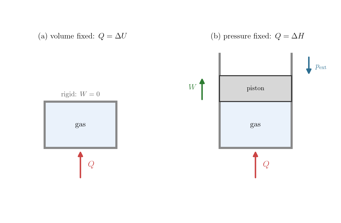
The internal energy and the enthalpy as heat functions. Take a closed system whose only work is expansion, and carry it from an initial equilibrium state to a final one. The first law \(\Delta U = Q - W\) fixes the heat \(Q\) absorbed over the process once the work \(W\) is known, and under two natural constraints (sketched in Figure 9.1) \(W\) follows from the endpoints alone, with no appeal to reversibility. If the volume is held fixed, in a rigid vessel, the boundary never moves, no work is done, and \[ Q = \Delta U \qquad (\text{volume fixed}). \] The internal energy is the heat absorbed at constant volume, the quantity whose temperature derivative is \(C_V\) (Lecture 3). If instead the boundary pressure is held at a constant value \(p_{\rm ext}\), and the system is in mechanical equilibrium with it at the two endpoints so that \(p = p_{\rm ext}\) there, the work done is \[ W = \int p_{\rm ext}\,dV = p_{\rm ext}\,\Delta V = \Delta(pV), \] the first equality because \(p_{\rm ext}\) is constant, the second because \(p = p_{\rm ext}\) at the endpoints. The first law then gives \[ Q = \Delta U + \Delta(pV) = \Delta(U + pV) = \Delta H \qquad (\text{pressure fixed}), \] so the enthalpy is the heat absorbed at constant pressure, the quantity behind \(C_p\). Both results are finite and rest only on the first law and the constancy of the constraint, never on \(\delta Q = T\,dS\), so they hold for irreversible processes too, a sudden reaction in an open flask no less than a slow warming. This, rather than its awkward natural variables \((S, p)\), is what recommends the enthalpy: it is the natural measure of heat in the constant-pressure processes of chemistry and the laboratory.
Heat functions — \(Q = \Delta U\) at constant volume, \(Q = \Delta H\) at constant pressure, for any process (reversible or not); these underlie \(C_V\) and \(C_p\).
The Helmholtz free energy and the maximum work. The second law turns the remaining two potentials into bounds, both read off the one apparatus of Figure 9.2. Let a closed system be in thermal contact with a single reservoir at temperature \(T_{\rm res}\), and carry it between an initial and a final equilibrium state both at the reservoir temperature, so that \(T = T_{\rm res}\) at each end. The first law \(\Delta U = Q - W\) and the Clausius inequality \(Q \le T_{\rm res}\,\Delta S\) (Lecture 7) together give \[ W = Q - \Delta U \le T_{\rm res}\,\Delta S - \Delta U = -\,\Delta F, \tag{9.11}\] where the last equality uses \(T = T_{\rm res}\) at both endpoints, so that \(T_{\rm res}\,\Delta S - \Delta U = -\Delta(U - TS) = -\Delta F\), with \(F = U - TS\) the Helmholtz free energy. Hence \(W \le -\Delta F\), with equality only for a reversible process: the most work a system can deliver in passing between two states at the reservoir temperature is the fall in its Helmholtz free energy, attained only in the reversible limit. The name records this. Of the energy \(U\), the part \(-\Delta F\) is free to leave as work, while the rest stays bound up with the entropy exchanged with the reservoir.
Maximum work — at constant temperature a system delivers at most \(W = -\Delta F\), the fall in its Helmholtz free energy, reached only reversibly.
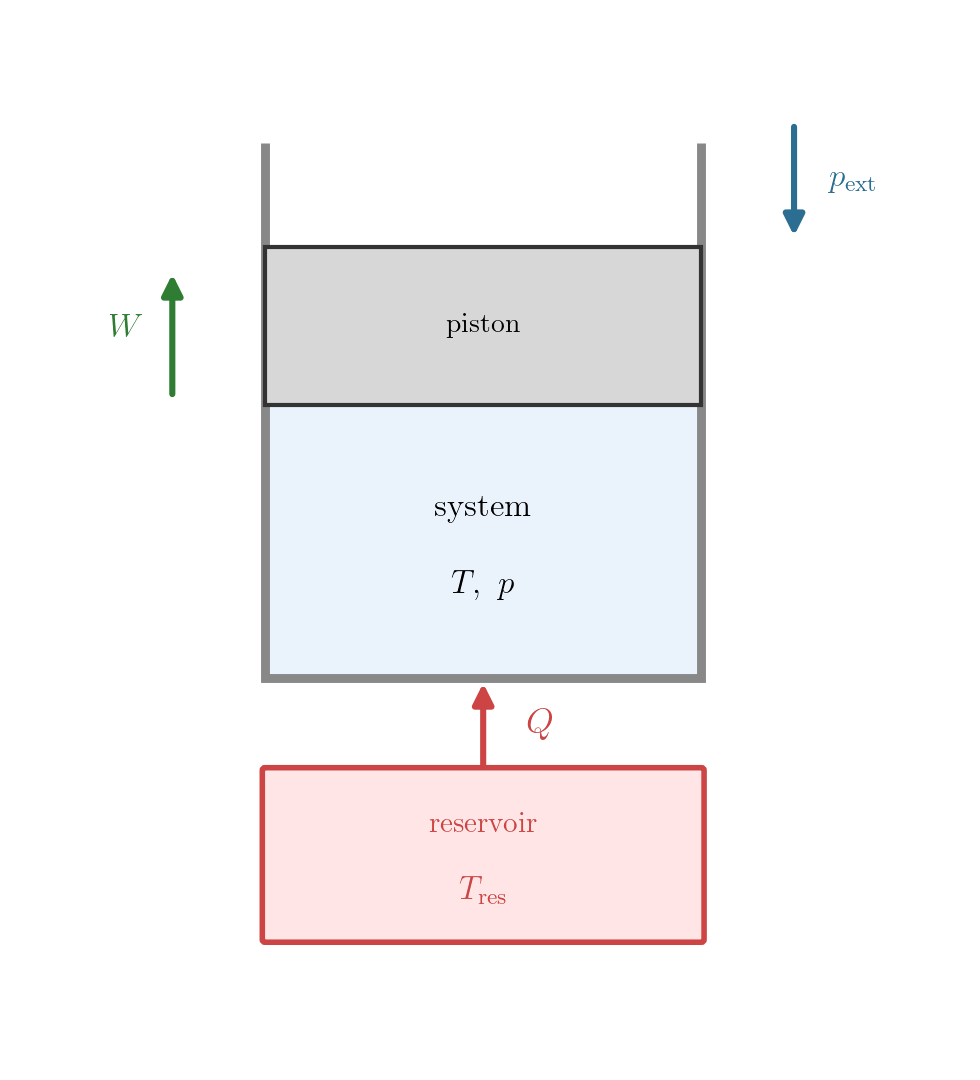
The Gibbs free energy and equilibrium. Hold the system at constant pressure as well. Let it be in thermal contact with the reservoir at \(T_{\rm res}\) and bear against a constant boundary pressure \(p_{\rm ext}\), with expansion its only work, and let the endpoints be in both thermal and mechanical equilibrium with the surroundings, so that \(T = T_{\rm res}\) and \(p = p_{\rm ext}\) at each end. The work is then \(W = p_{\rm ext}\,\Delta V\), and the first law with the Clausius inequality gives \[ \Delta U = Q - W \le T_{\rm res}\,\Delta S - p_{\rm ext}\,\Delta V . \] At the endpoints \(T_{\rm res}\,\Delta S = \Delta(TS)\) and \(p_{\rm ext}\,\Delta V = \Delta(pV)\), so this rearranges to \[ \Delta G \le 0 \qquad (\text{constant } T, p), \tag{9.12}\] with \(G = U - TS + pV\) the Gibbs free energy and equality only for a reversible step. A spontaneous process at constant temperature and pressure can therefore only lower \(G\), and the system comes to rest where \(G\) can fall no further: equilibrium at constant \(T\) and \(p\) is the state of minimum \(G\). This is no new principle but the law of increase of entropy in another guise. The fall in \(G\) is exactly \(T_{\rm res}\) times the entropy generated, \(\Delta G = -T_{\rm res}\,\Delta S_{\rm univ}\), counting system and reservoir together (Lecture 7); minimising \(G\) at constant \(T\) and \(p\) is just maximising the total entropy, the form the second law takes for a system in contact with surroundings rather than isolated.
Minimum Gibbs free energy — at constant \(T\) and \(p\), \(\Delta G \le 0\) in any spontaneous process, so equilibrium is the state of least \(G\); equivalently, the total entropy is greatest.
The chemical potential as molar Gibbs free energy. The Gibbs free energy is extensive, and for a one-component system it is a function of the intensive variables \(T\) and \(p\) and the extensive \(n\) alone; scaling \(n\) at fixed \(T\) and \(p\) scales \(G\) in proportion, so \(G = n\,g(T, p)\) with \(g = G/n\) the molar Gibbs free energy. Since \(g\) does not depend on \(n\), \[ \mu = \left(\frac{\partial G}{\partial n}\right)_{T,p} = g = \frac{G}{n}, \tag{9.13}\] and the chemical potential of a one-component system is its molar Gibbs free energy, the result anticipated in Lecture 8. The Euler relation Equation 9.3 says the same thing, \(G = U - TS + pV = \mu\,n\).
\(\mu = g\) — for one component the chemical potential is the molar Gibbs free energy, \(\mu = G/n\).
9.6 The Maxwell relations
Each of the four potentials is a state function, so its differential is exact, and for an exact differential the order of differentiation does not matter: the two mixed second derivatives are equal. Hold the composition \(n\) fixed, so that a potential \(\Phi\) is a function of its two remaining natural variables \(a\) and \(b\), with \(d\Phi = X\,da + Y\,db\) and \(X = (\partial\Phi/\partial a)_b\), \(Y = (\partial\Phi/\partial b)_a\). The equality of the mixed second derivatives, \(\partial^2\Phi/\partial b\,\partial a = \partial^2\Phi/\partial a\,\partial b\), forces a relation between the derivatives of the two coefficients, \[ \left(\frac{\partial X}{\partial b}\right)_a = \left(\frac{\partial Y}{\partial a}\right)_b , \] a Maxwell relation. Each of the four potentials yields one, with \(n\) held fixed throughout and therefore carried in every subscript below.
Maxwell relations — equalities among the derivatives of \(p\), \(V\), \(T\) and \(S\) that follow from the exactness of \(dU\), \(dH\), \(dF\), \(dG\); they trade derivatives of the entropy for derivatives of the equation of state.
Take the Helmholtz free energy as the worked case. From \(dF = -S\,dT - p\,dV\) at fixed \(n\), the coefficient of \(dT\) is \(-S = (\partial F/\partial T)_{V,n}\) and that of \(dV\) is \(-p = (\partial F/\partial V)_{T,n}\). Equating the mixed second derivative taken in either order gives \(-(\partial S/\partial V)_{T,n} = -(\partial p/\partial T)_{V,n}\), that is \((\partial S/\partial V)_{T,n} = (\partial p/\partial T)_{V,n}\). The same step on the other three potentials, each read off its differential in Table 9.1, gives the rest, each coefficient entering with its own sign: the relations from \(U\) and \(G\), which pair coefficients of opposite sign, carry a minus, while those from \(H\) and \(F\) do not. The four Maxwell relations are \[ \left(\frac{\partial T}{\partial V}\right)_{S,n} = -\left(\frac{\partial p}{\partial S}\right)_{V,n} \qquad (\text{from } U), \tag{9.14}\] \[ \left(\frac{\partial T}{\partial p}\right)_{S,n} = \left(\frac{\partial V}{\partial S}\right)_{p,n} \qquad (\text{from } H), \tag{9.15}\] \[ \left(\frac{\partial S}{\partial V}\right)_{T,n} = \left(\frac{\partial p}{\partial T}\right)_{V,n} \qquad (\text{from } F), \tag{9.16}\] \[ \left(\frac{\partial S}{\partial p}\right)_{T,n} = -\left(\frac{\partial V}{\partial T}\right)_{p,n} \qquad (\text{from } G). \tag{9.17}\] Differentiating in \(n\) as well would give further relations involving the chemical potential, which we shall not need here.
Their value is physical, not formal. The entropy is not something one measures directly, and neither are its derivatives; the right-hand sides, by contrast, are derivatives among \(p\), \(V\) and \(T\), which the equation of state supplies. The relations from \(F\) and \(G\) make this trade in its most useful form, turning \((\partial S/\partial V)_{T,n}\) and \((\partial S/\partial p)_{T,n}\) into \((\partial p/\partial T)_{V,n}\) and \(-(\partial V/\partial T)_{p,n}\); those from \(U\) and \(H\), which involve derivatives at constant entropy, complete the set. The \(F\)-relation Equation 9.16 is the one the next section uses to express the internal pressure \((\partial U/\partial V)_{T,n}\) through the equation of state.
9.7 The energy equation
The fundamental relation delivers the temperature and the pressure as derivatives of the internal energy, but it says nothing directly about how the energy depends on the volume at fixed temperature. That coefficient, \((\partial U/\partial V)_{T,n}\), has the units of a pressure and is called the internal pressure: it measures how the energy responds as the molecules are drawn apart, and it vanishes when they do not interact. It is also the coefficient that the first \(T\,dS\) equation of Lecture 7 (Equation 7.15) carried but left unevaluated, with the promise that the potentials would fix it. A Maxwell relation now does.
Regard the internal energy as a function of temperature and volume at fixed \(n\). Differentiating the fundamental relation \(dU = T\,dS - p\,dV\) with respect to \(V\) at constant \(T\) and \(n\) gives \[ \left(\frac{\partial U}{\partial V}\right)_{T,n} = T\left(\frac{\partial S}{\partial V}\right)_{T,n} - p . \] The entropy derivative on the right is not directly measurable; but the Maxwell relation from \(F\), Equation 9.16, replaces it with \((\partial p/\partial T)_{V,n}\), leaving the energy equation \[ \left(\frac{\partial U}{\partial V}\right)_{T,n} = T\left(\frac{\partial p}{\partial T}\right)_{V,n} - p . \tag{9.18}\] The internal pressure, a property of the energy, is thereby fixed entirely by the equation of state: knowing \(p\) as a function of \(T\) and \(V\) is enough to determine how the energy varies with volume.
Energy equation \((\partial U/\partial V)_{T,n} = T(\partial p/\partial T)_{V,n} - p\) — the internal pressure, fixed by the equation of state alone. Zero for an ideal gas, \(a n^2/V^2\) for a van der Waals gas.
Two cases show it at work. For an ideal gas, \(p = nRT/V\) gives \((\partial p/\partial T)_{V,n} = nR/V\), so \[ \left(\frac{\partial U}{\partial V}\right)_{T,n} = T\,\frac{nR}{V} - \frac{nRT}{V} = 0 : \] the internal energy depends on the temperature alone. In Lecture 4 this was read off Joule’s free-expansion experiment, an empirical input; here it follows from the equation of state \(pV = nRT\) through the energy equation. The two facts that lecture took as separate inputs are in truth linked: once the mechanical equation of state is granted, thermodynamics forces the internal energy to depend on the temperature alone, and the free expansion confirms this rather than supplying it independently. For a van der Waals gas, whose equation of state \(p = nRT/(V - nb) - a n^2/V^2\) is developed in the guided problem of this lecture, \((\partial p/\partial T)_{V,n} = nR/(V - nb)\), so \[ \left(\frac{\partial U}{\partial V}\right)_{T,n} = \frac{nRT}{V - nb} - \left(\frac{nRT}{V - nb} - \frac{a n^2}{V^2}\right) = \frac{a n^2}{V^2}, \] the internal pressure of the molecular attraction, positive because separating molecules that attract one another costs energy. This one line is all the lecture needs; the full internal energy \(U(T, V)\) and entropy \(S(T, V)\) are integrated from it in the guided problem.
The same identity can be reached without the potentials at all, by demanding that the differential \(dS\) read off the \(T\,dS\) equation Equation 7.15 be exact; the two routes agree.
9.8 Summary
Extensivity (first-order homogeneity of \(U\), Equation 9.2) gives the Euler relation \(U = TS - pV + \mu n\) (Equation 9.3).
Differentiating the Euler relation and subtracting the fundamental relation gives Gibbs–Duhem \(S\,dT - V\,dp + n\,d\mu = 0\) (Equation 9.4), per mole \(d\mu = -s\,dT + v\,dp\) (2): \(T,p,\mu\) are not independent, and \(\mu=\mu(T,p)\) for one component.
Legendre transforms of \(U\) produce potentials with controllable natural variables: \(H = U+pV\) (\(dH = T\,dS + V\,dp + \mu\,dn\), Equation 9.8), \(F = U-TS\) (\(dF = -S\,dT - p\,dV + \mu\,dn\), Equation 9.7), and \(G = U-TS+pV\) (\(dG = -S\,dT + V\,dp + \mu\,dn\), Equation 9.9).
Heat functions: \(U\) and \(H\) are the heat absorbed at constant volume and at constant pressure, \(Q=\Delta U\) and \(Q=\Delta H\) (behind \(C_V\) and \(C_p\)), reversibly or not.
Free energies and equilibrium: \(-\Delta F\) is the maximum work extractable at constant \(T\), reached reversibly (Equation 9.11); \(G\) is minimised at constant \(T\) and \(p\) (Equation 9.12); and for one component \(\mu=(\partial G/\partial n)_{T,p}=g=G/n\) (Equation 9.13), equivalently \(G=\mu n\).
The four Maxwell relations (Equation 9.14–Equation 9.17) follow from the equality of mixed second derivatives and trade entropy derivatives for \(p,V,T\) ones.
The energy equation \((\partial U/\partial V)_{T,n} = T(\partial p/\partial T)_{V,n} - p\)
- follows from the \(F\)-Maxwell relation; it gives \(0\) for the ideal gas and \(a n^2/V^2\) for the van der Waals gas (guided problem).
9.9 Problems
Problem 9.1 (Guided. The van der Waals gas was previewed in Problem 7.15 and Problem 7.16; here it is developed in full, and its results are cited in the energy-equation example of this lecture.) A van der Waals gas of \(n\) moles obeys the equation of state \[ \left(p + \frac{a n^2}{V^2}\right)(V - nb) = nRT, \] with constants \(a > 0\) and \(b > 0\) and molar heat capacity \(c_V\).
Solve for \(p(T,V)\) and interpret the two corrections to the ideal-gas law: the term \(-a n^2/V^2\) as the lowering of the pressure by the mutual attraction of the molecules, and \(nb\) as the volume they exclude. Recover \(pV = nRT\) in the limit \(a, b \to 0\).
Using the energy equation 1, show that the internal pressure is \[ \left(\frac{\partial U}{\partial V}\right)_{T,n} = \frac{a n^2}{V^2}. \]
Integrate at constant temperature, using \((\partial U/\partial T)_{V,n} = n\,c_V\), to obtain \[ U(T,V) = U_{\rm ideal}(T) - \frac{a n^2}{V}, \] with \(U_{\rm ideal}(T) = n\!\int c_V\,dT\) the ideal-gas internal energy. Interpret \(-a n^2/V\) as the potential energy stored in the attraction.
Using the first \(T\,dS\) equation Equation 7.15, show that the \(a\) terms cancel, leaving \(T\,dS = n\,c_V\,dT + \dfrac{nRT}{V - nb}\,dV\); for constant \(c_V\) this integrates to \[ S(T,V) = n\,c_V \ln T + nR\ln(V - nb) + \text{const}. \] Note the asymmetry: \(a\) enters the internal energy but not the entropy, while \(b\) enters the entropy but not the internal energy.
(More demanding.) The critical point is the state at which an isotherm has a horizontal inflection in the \((V,p)\) plane, \[ \left(\frac{\partial p}{\partial V}\right)_{T,n} = \left(\frac{\partial^2 p}{\partial V^2}\right)_{T,n} = 0. \] Solve these two conditions for the critical volume, temperature and pressure, \[ V_c = 3nb, \qquad T_c = \frac{8a}{27Rb}, \qquad p_c = \frac{a}{27 b^2}, \] and verify the substance-independent ratio \(p_c V_c/(nRT_c) = 3/8\). (Its meaning as the end of the liquid-vapour coexistence is taken up in Lecture 10.)
(More demanding.) In the reduced variables \(p_r = p/p_c\), \(V_r = V/V_c\), \(T_r = T/T_c\), show that the equation of state becomes \[ \left(p_r + \frac{3}{V_r^2}\right)\left(V_r - \tfrac{1}{3}\right) = \tfrac{8}{3}\,T_r, \] free of \(a\), \(b\) and \(n\): all van der Waals gases obey one and the same reduced equation of state (the law of corresponding states).
(Optional.) The gas expands freely into a vacuum from \(V_1\) to \(V_2\), doing no work and exchanging no heat. Since \(U\) is then unchanged, use part (c) and take \(c_V\) constant to show that the temperature falls by \[ \Delta T = -\frac{a n}{c_V}\left(\frac{1}{V_1} - \frac{1}{V_2}\right) < 0 , \] the cooling on free expansion (the Joule effect) that the ideal gas does not show.
Problem 9.2 The Gibbs free energy of \(n\) moles of an ideal gas can be written \[ G(T,p,n) = n\big[\,g_0(T) + RT\ln(p/p_0)\,\big], \] with \(p_0\) a reference pressure and \(g_0(T)\) a function of temperature alone.
Using the differential \(dG = -S\,dT + V\,dp + \mu\,dn\) (Equation 9.9), compute \(V\), \(S\) and \(\mu\) as the derivatives of \(G\).
Verify that \(V\) reproduces the equation of state \(pV = nRT\), and that \(\mu = (\partial G/\partial n)_{T,p} = g = G/n\) (Equation 9.13) recovers the ideal-gas chemical potential Equation 8.9.
Problem 9.3 For \(n\) moles of an ideal gas with constant molar heat capacity \(c_V\) (internal energy \(U = n\,c_V T\) up to a constant, equation of state \(pV = nRT\)):
Write the enthalpy \(H = U + pV\), the Helmholtz free energy \(F = U - TS\) and the Gibbs free energy \(G = U - TS + pV\) as combinations of \(U\), the ideal-gas entropy \(S\) of Lecture 7 and the equation of state, and state the differential and the natural variables of each (Table 9.1). Show in particular that \(H = n\,c_p T\) with \(c_p = c_V + R\).
From \(dF = -S\,dT - p\,dV + \mu\,dn\), confirm that \(-p = (\partial F/\partial V)_{T,n}\) reproduces \(pV = nRT\).
Problem 9.4
For \(n\) moles of an ideal gas, compute both sides of the \(F\)-Maxwell relation \((\partial S/\partial V)_{T,n} = (\partial p/\partial T)_{V,n}\) (Equation 9.16) and verify that they agree.
Using the \(G\)-Maxwell relation \((\partial S/\partial p)_{T,n} = -(\partial V/\partial T)_{p,n}\) (Equation 9.17), compute \((\partial S/\partial p)_{T,n}\) for the ideal gas and integrate at constant temperature to recover the pressure dependence of the entropy, \(S(T,p) - S(T,p_0) = -nR\ln(p/p_0)\).
Problem 9.5
For a one-component system the per-mole Gibbs–Duhem relation reads \(d\mu = -s\,dT + v\,dp\) (2). For an ideal gas, with molar volume \(v = RT/p\), integrate this at constant temperature to recover \[ \mu(T,p) = \mu(T,p_0) + RT\ln(p/p_0), \] the result Equation 8.9.
Verify that \(G = \mu n\) (Equation 9.13), the form the Euler relation Equation 9.3 takes for the Gibbs free energy, for the ideal gas: compute \(U - TS + pV\) from the molar energy and entropy and show it equals \(n\mu\), with \(\mu = u + RT - Ts\) (Equation 8.8).
Problem 9.6 \(n\) moles of an ideal gas at temperature \(T\), in thermal contact with a reservoir at the same temperature, are expanded from \(V_1\) to \(V_2 = 2V_1\).
Compute the change \(\Delta F\) in the Helmholtz free energy between the two states, and hence the maximum work \(-\Delta F\) the gas can deliver at this temperature (Equation 9.11).
Compute the work actually done by the gas on a reversible isothermal expansion, and on a sudden expansion against a constant boundary pressure \(p_{\rm ext} = nRT/V_2\). Compare each with \(-\Delta F\) and identify the work lost in the irreversible case.
Problem 9.7 A gas of \(n\) moles obeys the co-volume equation of state \(p = nRT/(V - nb)\), with \(b\) a constant (the van der Waals gas of Problem 9.1 with \(a = 0\); see also Problem 7.15).
Using the energy equation 1, show that \((\partial U/\partial V)_{T,n} = 0\), so that the internal energy depends on the temperature alone, exactly as for an ideal gas.
Explain physically why the excluded volume \(b\) leaves the internal energy independent of volume, whereas the attraction \(a\) of Problem 9.1 does not: \(b\) changes the pressure but stores no energy of interaction.
Problem 9.8 (More demanding.)
Combine the relation \(C_p - C_V = \big[\,p + (\partial U/\partial V)_{T,n}\,\big](\partial V/\partial T)_{p,n}\) (Equation 3.12, Lecture 3) with the energy equation 1 to show that \[ C_p - C_V = T\left(\frac{\partial p}{\partial T}\right)_{V,n}\left(\frac{\partial V}{\partial T}\right)_{p,n}. \]
Verify that this gives \(C_p - C_V = nR\) for the ideal gas.
Take as given the cyclic relation among \(p\), \(V\), \(T\) at fixed \(n\), \((\partial V/\partial T)_{p,n} = -(\partial p/\partial T)_{V,n}\big/(\partial p/\partial V)_{T,n}\). Using it together with the isothermal compressibility \(\kappa_T = -\tfrac1V(\partial V/\partial p)_{T,n}\) (Lecture 8), rewrite the result as \[ C_p - C_V = T V \kappa_T \left(\frac{\partial p}{\partial T}\right)_{V,n}^{\!2} \ge 0 , \] and conclude that \(C_p \ge C_V\) for every substance, with equality only when \((\partial p/\partial T)_{V,n} = 0\).
Problem 9.9 (Forward-looking: previews Lecture 10.) A pure substance can exist in more than one phase, for instance liquid and vapour, each a homogeneous form of the substance with its own molar Gibbs free energy \(g(T,p)\).
At given \(T\) and \(p\) the substance settles into whichever phase has the lower \(g\) (the \(G\)-minimum principle Equation 9.12 applied to \(G = n g\)). Argue that two phases can coexist only where their molar Gibbs free energies are equal, \(g_1(T,p) = g_2(T,p)\), which is the diffusive-equilibrium condition \(\mu_1 = \mu_2\) of Lecture 8 (recall \(\mu = g\), Equation 9.13).
The equation \(g_1(T,p) = g_2(T,p)\) defines a coexistence curve \(p(T)\). Differentiating it along the curve and using the per-mole Gibbs–Duhem relation \(dg = -s\,dT + v\,dp\)
- for each phase, show that \[ \frac{dp}{dT} = \frac{s_2 - s_1}{v_2 - v_1}, \] with \(s_i\), \(v_i\) the molar entropy and volume of the two phases. (This is the Clausius–Clapeyron relation, derived in Lecture 10.)