3 Thermal Equilibrium and Empirical Temperature
Part I — Foundations
Last updated: 01-06-2026
3.1 Properties of thermal equilibrium and thermalization process
We recall that “placing two systems in thermal contact” means to allow them to exchange heat but neither matter nor work. Two systems in separate thermodynamic equilibrium are said to be in mutual thermal equilibrium if, once placed in thermal contact, no macroscopic changes occur in either system. The following principles based on empirical observations specify the properties of thermal equilibrium and describe how thermal equilibrium is reached. They are the basis for the definition of temperature and for the formulation of the Second Law of Thermodynamics.
P 3.1 (Zeroth Law of Thermodynamics) Consider three systems \(A\), \(B\) and \(C\) in separate thermodynamic equilibrium. If \(A\) is in thermal equilibrium with \(B\), and \(B\) is in thermal equilibrium with \(C\), then \(A\) is in thermal equilibrium with \(C\). That is, the property of being in mutual thermal equilibrium is transitive.
P 3.2 Consider two systems \(A\) and \(B\) in separate thermodynamic equilibrium, but not in mutual thermal equilibrium. When they are placed in thermal contact, they will exchange heat spontaneously until they reach thermal equilibrium. The process of reaching thermal equilibrium is called thermalization. We will say that, during thermalization heat flows from \(A\) to \(B\) if the internal energy of \(A\) decreases and the internal energy of \(B\) increases, while heat flows from \(B\) to \(A\) if the internal energy of \(B\) decreases and the internal energy of \(A\) increases. The direction of the heat flow is completely determined by the initial states of \(A\) and \(B\) and it does not depend on the details of the thermalization process. One could say that if heat is observed to flow from \(A\) to \(B\) in a particular thermalization process, a thermalization process in which the heat flows from \(B\) to \(A\) is physically impossible.
P 3.3 Consider four systems \(A\), \(A'\), \(B\) and \(B'\) in separate thermodynamic equilibrium, such that \(A\) is in thermal equilibrium with \(A'\), while \(B\) is in thermal equilibrium with \(B'\). If heat flows from \(A\) to \(B\) when the two systems are placed in thermal contact, then heat flows from \(A'\) to \(B'\) when they are placed in thermal contact as well.
P 3.4 Consider three systems \(A\), \(B\) and \(C\) in separate thermodynamic equilibrium. If heat flows from \(A\) to \(B\) when they are placed in thermal contact, and from \(B\) to \(C\) when they are placed in thermal contact, then heat flows from \(A\) to \(C\) when they are placed in thermal contact as well.
The Zeroth Law usually plays a prominent role in standard textbooks and Principle 3.2 is often incorporated in the formulation of the Second Law. The other principles are often not spelled out and invoked as hidden assumptions. I have chosen to state these principles explicitly and to give them equal importance at this stage, because they all play a crucial role in the definition of temperature. With the definition of temperature in hand, we will be able to give a sharper enunciation of the Second Law in Lecture 5.
3.2 Definition of empirical temperature
Essentially, a scale of empirical temperature is defined by means of a thermometer. This definition is not universal, but different thermometers will generally yield different temperature scales. The concept of absolute temperature will be introduced later on, and it is a universal concept that does not depend on the choice of thermometer. But let us focus on empirical temperature for now.
A thermometer is a thermodynamic system that can exchange heat but not work with the environment and has some measurable property \(\tau\) which satisfies the following conditions: (1) two identical thermometers are in thermal equilibrium if and only if they have the same value of \(\tau\), (2) \(\tau\) is a strictly increasing continuous function of its internal energy. The chosen property is called the thermometric property. A temperature scale is specified by choosing a strictly increasing continuous function \(\theta(\tau)\) of the thermometric property. When the thermometer is in thermodynamic equilibrium, the value of \(\theta(\tau)\) is called the reading of the thermometer.
Thermometer — a system that exchanges only heat with its surroundings and has a thermometric property \(\tau\) that is a strictly increasing function of its internal energy.
Given a system in thermodynamic equilibrium, we define its empirical temperature \(\theta\) as the reading of a thermometer that is in thermal equilibrium with the system. We will say that a system A in thermodynamic equilibrium is hotter (resp. colder) than a system B in thermodynamic equilibrium if the empirical temperature of A is greater (resp. smaller) than the empirical temperature of B.
3.2.1 Properties of empirical temperature
Empirical temperature \(\theta\) — the reading of a thermometer in thermal equilibrium with the system. Unique, uniform, and intensive; depends on the choice of thermometer.
We prove now a number of important properties that any definition of empirical temperature must satisfy as well as the statement that what is hotter and colder does not depend on the choice of thermometer. These properties are consequences of the definition of empirical temperature and of the principles of thermal equilibrium stated in Section 3.1.
C 3.1 The empirical temperature of a system in thermodynamic equilibrium is uniquely defined and is uniform across the system.
Proof – There are two potential issues in the operational definition of empirical temperature. First, we need to make sure that two replicas of the thermometer will measure the same temperature. This is straightforward: if two identical thermometers are in thermal equilibrium with the same system, they will be in thermal equilibrium with each other (Principle 3.1), and therefore they will read the same temperature.
There is a second more subtle point. Thermodynamic systems are typically extended. We measure the temperature by placing the thermometer in contact with the system, however we could place the thermometer in contact with the system in different points. For the definition of temperature to make sense, the thermometer should always read the same temperature. We want to prove this.
Consider a system \(A\) in thermodynamic equilibrium enclosed in a certain volume. Divide the volume in small cells and consider the subsystems \(S_1\), \(S_2\)… defined as the portions of the system enclosed in each cell. \(A\) is in thermodynamic equilibrium, no macroscopic changes can occur over time, in particular no net fluxes of matter, heat and work can exist between any pair of contiguous subsystems. Therefore all subsystems are in mutual thermal equilibrium. If the thermometer is in thermal equilibrium with any of them, it is in thermal equilibrium with all of them thanks to the Zeroth Law (Principle 3.1). Therefore the thermometer will read the same temperature when placed in thermal contact with different parts of the system.
C 3.2 The empirical temperature is intensive.
Proof – As proved in the previous point, each part of the system has the same temperature of the whole system, i.e. the temperature does not change with the size of the system.
C 3.3 Two systems are in mutual thermal equilibrium if and only if they have the same empirical temperature.
Proof – Consider two systems in mutual thermal equilibrium. Thanks to the Zeroth Law (Principle 3.1), a thermometer that is in thermal equilibrium with one of the two systems will also be in thermal equilibrium with the other system, and therefore the reading of the thermometer will be the same for both systems, meaning they have the same empirical temperature.
On the other hand, consider two systems with the same temperature \(\theta\). This means that a thermometer reading \(\theta\) is in mutual thermal equilibrium with both systems. Thanks to the Zeroth Law (Principle 3.1), the two systems are in mutual thermal equilibrium.
C 3.4 Consider two systems in separate thermodynamic equilibrium but not in mutual thermal equilibrium. When placed in thermal contact, heat flows spontaneously from the hotter system to the colder one. In particular, the definition of what is hotter and what is colder does not depend on the choice of thermometer.
Proof – From the definition of thermometer, it follows that a strictly increasing continuous function \(U = f_{\mathcal{T}}(\theta)\) exists between the reading of the thermometer and its internal energy.
Let \(H\) be the hotter system with temperature \(\theta_H\) and let \(C\) be the colder system with temperature \(\theta_C < \theta_H\). Consider now two identical thermometers \(\mathcal{T}_H\) and \(\mathcal{T}_C\) in thermal equilibrium with \(H\) and \(C\), respectively. Then, their internal energies are \(U_H = f_{\mathcal{T}}(\theta_H)\) and \(U_C = f_{\mathcal{T}}(\theta_C)\). Since \(f_{\mathcal{T}}\) is a strictly increasing function, it follows that \(U_H > U_C\).
We place now the two thermometers in thermal contact. During the thermalization process they exchange heat \(Q\) defined with the following sign convention: \(Q>0\) means that heat flows from \(H\) to \(C\), while \(Q<0\) means that heat flows from \(C\) to \(H\). At the end of the thermalization process the two thermometers have energy \(U'_H = U_H - Q\) and \(U'_C = U_C + Q\). Since the two thermometers are now in equilibrium, they read the same temperature which implies that they have the same internal energy, i.e. \(U_H - Q = U'_H = U'_C = U_C + Q\). Solving for the transferred heat one finds \(Q = (U_H - U_C)/2 > 0\), since \(U_H > U_C\). Therefore, heat flows spontaneously from \(\mathcal{T}_H\) to \(\mathcal{T}_C\). Thanks to Principle 3.3, heat flows spontaneously from the hotter system \(H\) to the colder system \(C\) when the two systems are placed in thermal contact.
C 3.5 Given two empirical temperature scales defined by two thermometers \(\mathcal{T}\) and \(\mathcal{T}'\). A conversion function \(C_{\mathcal{T}' \leftarrow \mathcal{T}}\) exists between the two temperature scales, defined by the property that the thermometer \(\mathcal{T}\) with reading \(\theta\) is in thermal equilibrium with the thermometer \(\mathcal{T}'\) with reading \(\theta' = C_{\mathcal{T}' \leftarrow \mathcal{T}}(\theta)\). The conversion function is strictly increasing.
Proof – See Problem 3.6.
3.3 Examples of thermometers
3.3.1 The mercury thermometer
A simple example is given by a mercury thermometer which consists of a glass tube with a bulb at the end filled with mercury, while the rest of the tube is in a vacuum. In this case, the thermometric property is the height \(h\) of the mercury column in the tube. When the thermometer absorbs heat from the environment, the mercury expands and rises in the tube, i.e. \(h\) increases. On the other hand, when the thermometer releases heat to the environment, the mercury contracts and falls in the tube, i.e. \(h\) decreases. Notice that, while the volume of the mercury changes, the thermometer does not perform work on the environment since the pressure is zero. Therefore the thermometer exchanges only heat with the environment.
One can define the reading of the thermometer as the height of the mercury column itself (in this case the temperature would be measured in meters!) or, more generally, as a function of the height of the mercury column given in some arbitrary unit. Throughout the 19th century and half the 20th century, the Celsius scale was exactly defined by means of a mercury thermometer, in the following way. Let \(h_0\), resp. \(h_{100}\), be the height of the mercury column when the thermometer is in thermal equilibrium with water at its melting point, resp. boiling point, at standard atmospheric pressure. Then the Celsius temperature \(\theta_{\rm C}\) associated to a generic height \(h\) of the mercury column is defined as: \[ \theta_{\rm C} = \frac{h - h_0}{h_{100} - h_0} \times 100^{\,\circ}\mathrm{C} \ . \tag{3.1}\] Today, the Celsius scale is defined in terms of the Kelvin scale, which we will introduce later on. However, the definition of the Celsius scale in terms of a mercury thermometer is still useful as a pedagogical example of how to define a temperature scale based on a thermometric property.
3.3.2 The ideal gas thermometer
A gas thermometer consists of a fixed quantity of gas enclosed in a rigid container connected to a pressure gauge. Since the container is rigid, the volume of the gas is constant: \(dV = 0\) at every instant, and no \(p\,dV\) work is exchanged with the environment. The thermometric property is the pressure \(p\) of the enclosed gas. When the thermometer absorbs heat, the pressure rises; when it releases heat, the pressure falls.
In principle, one could use the pressure itself as definition of temperature, in which case the temperature would be measured in Pascals. However, it is more common to define the reading of the thermometer as an affine function of the pressure, and to choose two convenient reference points to calibrate the scale.
While one could also use in this case the melting and boiling points of water at standard atmospheric pressure as reference points to define the temperature scale in complete analogy with Equation 3.1, we want to discuss a different choice which is more in line with modern metrology.
One observes that the pressure is a non-negative quantity. It is natural to declare that zero pressure corresponds to zero temperature (this is the first reference point) and to choose a temperature scale that is proportional to the pressure. Only one more reference point is needed to fix the proportionality constant between temperature and pressure. The standard choice is given by the triple point of water: the unique thermodynamic state at which liquid water, ice, and water vapour coexist in equilibrium. This state occurs at a pressure of \(611.7\ \mathrm{Pa}\) and at a single value of the temperature (as defined e.g. by means of a mercury thermometer). Any small perturbations in the pressure or the temperature will cause one of the three phases to disappear.
The quantity \(p_{\rm tr}\) is defined as the pressure of the gas when the thermometer is in thermal equilibrium with water at its triple point. Then one chooses a conventional temperature value \(\theta_{\rm tr}\) for the triple point, and defines the gas-thermometer scale by requiring that the temperature is proportional to the pressure: \[ \theta_{\rm G} = \frac{p}{p_{\rm tr}}\,\theta_{\rm tr}. \tag{3.2}\]
Triple point of water — the unique state at which liquid water, ice, and water vapour coexist in equilibrium. Used as a universal, reproducible calibration point for temperature scales.
Notice that \(\theta_{\rm tr}\) is an arbitrary constant that can be chosen at will. This arbitrariness is irreducible and it corresponds to the arbitrariness in defining the unit of measure for temperature. Different values of \(\theta_{\rm tr}\) yield different temperature scales, which are trivially related by a simple rescaling.
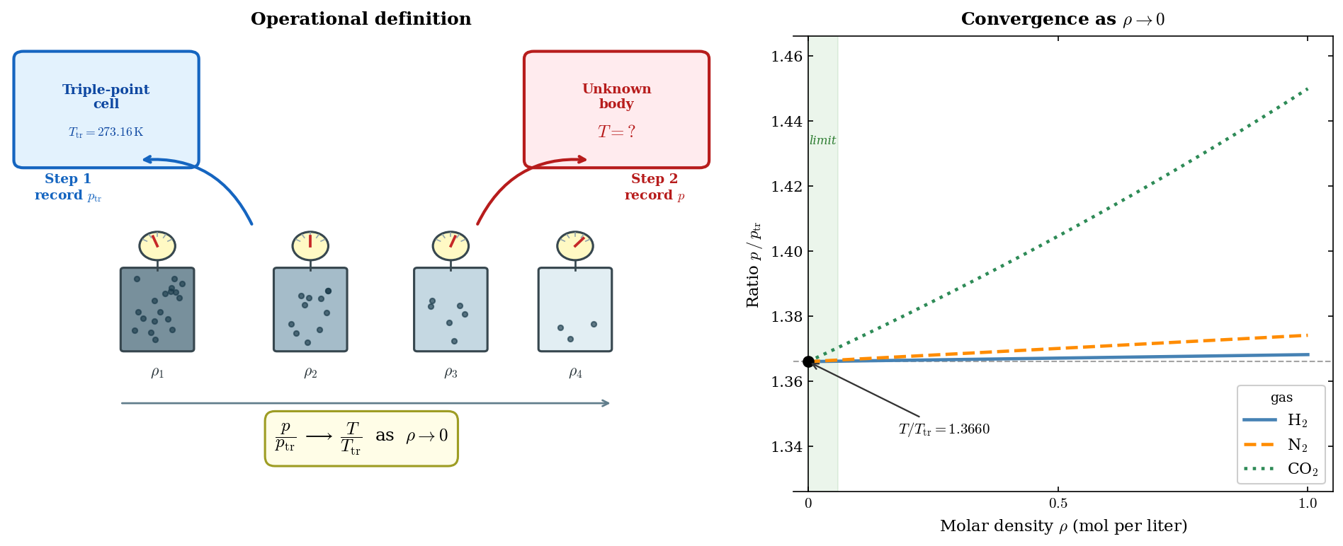
Gas thermometers that differ by the choice of the gas, the volume of the container or the amount of gas will yield different temperature scales. They will all read the same temperature \(\theta_{\rm tr}\) for the triple point of water, but they will generally differ for other states. Something remarkable occurs, however, when we make the gas more and more dilute. As the density \(\rho\) of the gas is reduced, the readings of thermometers filled with different gases are found to agree more and more closely at all intermediate temperatures. In the limit of zero density, all gas thermometers, regardless of the gas employed, give identical readings.
The zero-density limit for a gas is called the ideal gas limit. We reserve the symbol \(T\) for the temperature defined in this limit, to distinguish it from the finite-density reading \(\theta_{\rm G}\). \(T\) will also serve later as the symbol for absolute temperature; we will prove that the two coincide. The ideal gas temperature is defined as: \[ T = \lim_{\rho \to 0} \frac{p}{p_{\rm tr}} \times 273.16\ \mathrm{K} \ , \tag{3.3}\] where \(273.16\ \mathrm{K}\) is the conventional temperature assigned to the triple point of water, implicitly defining the kelvin as the unit of temperature. Notice that \(T\) is non-negative by definition.
With the kelvin fixed, the modern Celsius scale is also fully determined: it is the kelvin scale shifted by \(273.15\ \mathrm{K}\), \[ \theta_{\rm C} = T - 273.15\ \mathrm{K}, \tag{3.4}\] with the same degree size.
Ideal gas temperature \(T\) — the zero-density limit of the gas thermometer reading. Universal: independent of the gas used. Coincides with the absolute temperature (proved in Lecture 6).
Operational procedure. We prepare a series of containers of fixed volume, all filled with the same gas but to successively lower densities \(\rho_1 > \rho_2 > \rho_3 > \cdots\), each fitted with a manometer. The measurement proceeds in two steps.
Step 1. Place all containers in thermal contact with a triple-point cell. Allow equilibrium to be reached. Record the pressure \(p_{{\rm tr},i}\) for container \(i\).
Step 2. Place all containers in thermal contact with the body whose temperature is to be determined. Allow equilibrium. Record the pressure \(p_i\) for container \(i\).
Form the ratio \(r_i = p_i / p_{{\rm tr},i}\) for each container and observe how it depends on density:
3.4 Heat capacities
The heat capacity of a system is the ratio of the heat absorbed to the resulting temperature change in an infinitesimal process. Since \(\delta Q\) is path-dependent, we must specify the conditions under which the heat is supplied. In what follows we restrict attention to fluids, for which the only work term is \(p\,dV\); the definitions generalise to other systems by replacing the volume constraint with the appropriate work constraint. The amount of substance \(n\) is held fixed throughout, as we are dealing with closed systems.
The heat capacity at constant volume, \(C_V\) (in J K\(^{-1}\)), is defined by \[ C_V = \left( \frac{\delta Q}{dT} \right)_V. \tag{3.5}\] At constant volume, \(dV = 0\) and hence \(\delta W = p \, dV = 0\). The First Law gives \(\delta Q = dU\), so \[ C_V = \left( \frac{\partial U}{\partial T} \right)_V. \tag{3.6}\]
Heat capacity at constant volume \(C_V = (\partial U/\partial T)_V\). Heat capacity at constant pressure \(C_p = (\partial U/\partial T)_p + p(\partial V/\partial T)_p\). Both in J K\(^{-1}\); both extensive.
The heat capacity at constant pressure, \(C_p\) (in J K\(^{-1}\)), is defined by \[ C_p = \left( \frac{\delta Q}{dT} \right)_p. \tag{3.7}\] At constant pressure, \(\delta W = p \, dV\) and the First Law gives \(\delta Q = dU + p \, dV\), so \[ C_p = \left( \frac{\partial U}{\partial T} \right)_p + p\left( \frac{\partial V}{\partial T} \right)_p. \tag{3.8}\] Both \(C_V\) and \(C_p\) are extensive quantities: they scale proportionally with the amount of substance. The corresponding intensive quantities are the molar heat capacities (in J mol\(^{-1}\) K\(^{-1}\)), obtained by dividing by \(n\): \[ c_V = \frac{C_V}{n}, \qquad c_p = \frac{C_p}{n}, \tag{3.9}\] and the specific heat capacities (in J kg\(^{-1}\) K\(^{-1}\)), obtained by dividing by the total mass \(m = nM\), where \(M\) (in kg mol\(^{-1}\)) is the molar mass: \[ \tilde{c}_V = \frac{C_V}{m} = \frac{c_V}{M}, \qquad \tilde{c}_p = \frac{C_p}{m} = \frac{c_p}{M}. \tag{3.10}\] The heat capacity ratio or adiabatic index is a convenient quantity defined as \[ \gamma = \frac{C_p}{C_V} = \frac{c_p}{c_V} = \frac{\tilde{c}_p}{\tilde{c}_V} . \tag{3.11}\]
Adiabatic index \(\gamma = C_p/C_V\). For an ideal gas \(\gamma > 1\); for monatomic gases \(\gamma \approx 5/3\), for diatomic gases \(\gamma \approx 7/5\) near room temperature.
3.5 Summary
Thermal equilibrium and temperature
- Four empirical principles govern thermal equilibrium: transitivity (Zeroth Law), determinacy of heat-flow direction, equivalence of systems in mutual equilibrium, and transitivity of heat-flow direction. Together they are the foundation for the definition of temperature.
- A thermometer is a system that exchanges only heat with its surroundings and has a thermometric property \(\tau\) that is a strictly increasing function of its internal energy. A temperature scale is any strictly increasing function \(\theta(\tau)\).
- The empirical temperature \(\theta\) of a system is the reading of any thermometer in thermal equilibrium with it. It is uniquely defined, uniform across the system, and intensive. Two systems are in mutual thermal equilibrium if and only if they have the same empirical temperature; heat flows from the hotter to the colder.
Examples of thermometers
- The mercury thermometer uses column height as thermometric property. The historical Celsius scale fixed two reference points (melting and boiling of water at standard pressure): \(\theta_{\rm C} = (h - h_0)/(h_{100} - h_0) \times 100\,^\circ\mathrm{C}\).
- The gas thermometer uses pressure at fixed volume as thermometric property. The scale \(\theta_{\rm G} = (p/p_{\rm tr})\,\theta_{\rm tr}\) depends on the gas and its density, but in the zero-density limit all gases agree. This universal limit defines the ideal gas temperature \(T = \lim_{\rho\to 0}(p/p_{\rm tr})\times 273.16\ \mathrm{K}\), with the kelvin fixed by assigning \(273.16\ \mathrm{K}\) to the triple point of water.
Heat capacities
- The heat capacity at constant volume: \(C_V = (\partial U/\partial T)_V\).
- The heat capacity at constant pressure: \(C_p = (\partial U/\partial T)_p + p(\partial V/\partial T)_p\).
- Both are extensive; the corresponding intensive quantities are the molar heat capacities \(c_V = C_V/n\), \(c_p = C_p/n\), and the specific heat capacities \(\tilde{c}_V = c_V/M\), \(\tilde{c}_p = c_p/M\).
- The heat capacity ratio (adiabatic index): \(\gamma = C_p/C_V\).
3.6 Problems
Problem 3.1 Two gas thermometers use the same gas and setup but assign different conventional temperatures to the triple point: \(\theta_{\rm tr}\) and \(\theta_{\rm tr}'\) respectively. Show that the two scales are proportional everywhere: \(\theta_{\rm G}' = (\theta_{\rm tr}'/\theta_{\rm tr})\,\theta_{\rm G}\).
Problem 3.2 Using Equation 3.4, show that the numerical values of \(C_V\) and \(C_p\) are the same whether temperature is measured in kelvin or degrees Celsius.
Problem 3.3 Two fictitious liquid thermometers A and B are calibrated via Equation 3.1 at the melting point and the boiling point of water at standard atmospheric pressure. The melting point corresponds to \(h_A = 10\ \mathrm{cm}\) and the boiling point to \(h_A = 20\ \mathrm{cm}\). When placed in mutual thermal equilibrium, their column heights \(h_A\) and \(h_B\) (in cm) are related by \[ h_B = h_A^2 / (10\ \mathrm{cm}) . \]
Show that by construction the two thermometers agree at the two calibration points.
Compute the Celsius readings \(\theta_{\rm C}^{(A)}\) and \(\theta_{\rm C}^{(B)}\) at the state for which \(h_A = 15\ \mathrm{cm}\), and verify that the two readings disagree.
Identify the necessary and sufficient condition on the relation \(h_B(h_A)\) for the two thermometers to agree at every state in the calibration range.
Problem 3.4 Using Equation 3.6 and Equation 3.8, show that \[ C_p - C_V = \left[p + \left(\frac{\partial U}{\partial V}\right)_T\right]\left(\frac{\partial V}{\partial T}\right)_p. \tag{3.12}\]
Problem 3.5 The Gibbs phase rule states that a system of \(C\) chemical components with \(P\) coexisting phases has \(F = C - P + 2\) thermodynamic degrees of freedom (\(F\) counts the number of intensive thermodynamic variables that can be varied independently while keeping all \(P\) phases in coexistence). Use it to show that for a pure substance (\(C = 1\)), the coexistence of three phases fixes both temperature and pressure uniquely, which justifies the use of the triple point as a reproducible calibration standard.
Problem 3.6 Let \(\mathcal{T}\) and \(\mathcal{T}'\) be two thermometers with thermometric properties \(\tau\) and \(\tau'\) and temperature scales \(\theta(\tau)\) and \(\theta'(\tau')\), respectively. (i) Show that, for each reading \(\theta\) of \(\mathcal{T}\), there is a unique reading \(\theta'\) of \(\mathcal{T}'\) such that \(\mathcal{T}\) and \(\mathcal{T}'\) are in mutual thermal equilibrium, so that the conversion function \(C_{\mathcal{T}' \leftarrow \mathcal{T}}(\theta) = \theta'\) is well defined. (ii) Show that \(C_{\mathcal{T}' \leftarrow \mathcal{T}}\) is strictly increasing.
Problem 3.7 Three gas thermometers are filled with the same gas at decreasing densities \(\rho_1 > \rho_2 > \rho_3\). When placed in contact with a body of unknown temperature, they record pressures \(p_i\); when placed in contact with a triple-point cell, they record pressures \(p_{{\rm tr},i}\). The ratios \(r_i = p_i / p_{{\rm tr},i}\) are found to be \(1.3650\), \(1.3644\), and \(1.3640\) at densities \(\rho_i = 1.0,\ 0.5,\ 0.25\ \mathrm{mol\,L^{-1}}\) respectively. Assuming the ratios depend linearly on density in this range, extrapolate to zero density and determine the ideal gas temperature of the body.
Problem 3.8 Three gas thermometers are filled with different gases (He, \(\mathrm{N_2}\), \(\mathrm{CO_2}\)), each at the same molar density \(\rho = 1.0\ \mathrm{mol\,L^{-1}}\). When placed in contact with a body of unknown temperature, the recorded ratios \(r_i = p_i / p_{{\rm tr},i}\) are \[ r_{\rm He} = 1.3658, \qquad r_{\mathrm{N_2}} = 1.3651, \qquad r_{\mathrm{CO_2}} = 1.3625. \] The same measurement repeated at \(\rho = 0.1\ \mathrm{mol\,L^{-1}}\) gives \[ r_{\rm He}' = 1.3645, \qquad r_{\mathrm{N_2}}' = 1.3644, \qquad r_{\mathrm{CO_2}}' = 1.3642. \]
Using Equation 3.2 with \(\theta_{\rm tr} = 273.16\ \mathrm{K}\), compute the apparent temperature reading from each gas at each density.
The three readings disagree at \(\rho = 1.0\ \mathrm{mol\,L^{-1}}\) but nearly agree at \(\rho = 0.1\ \mathrm{mol\,L^{-1}}\). Explain why, and estimate the ideal-gas temperature \(T\) of the body by extrapolating each gas’s pair of readings linearly to \(\rho \to 0\). Verify that the three extrapolations agree.
Problem 3.9 An ideal gas obeys the equation of state \(pV = nRT\). We take as given that its internal energy depends only on temperature, \(U = U(T)\) — this property will be established in Lecture 4 from Joule’s free-expansion experiment, and is assumed here. A photon gas obeys \(p = \tfrac{1}{3}aT^4\) and \(U = aVT^4 = 3pV\).
Apply Equation 3.12 to the ideal gas. Using \(U = U(T)\) to compute \((\partial U/\partial V)_T\), and \(V = nRT/p\) to compute \((\partial V/\partial T)_p\), derive Mayer’s relation \[ C_p - C_V = nR. \]
Apply Equation 3.12 to the photon gas. Compute \((\partial U/\partial V)_T\) and the bracket \(\bigl[p + (\partial U/\partial V)_T\bigr]\). Show that \((\partial V/\partial T)_p\) is not defined: at constant \(p\), the equation of state \(p = \tfrac{1}{3}aT^4\) forces \(T\) to a single value, so no process at constant \(p\) has \(dT \neq 0\).
Using the definition of \(C_p\) in Equation 3.7, identify which step of the definition fails for the photon gas. Connect your answer to the observation in Problem 2.11 that the isobaric step of a photon-gas process is automatically isothermal.
Problem 3.10 A gas thermometer is calibrated using two reference points: the melting point and the boiling point of water at standard atmospheric pressure, assigned the conventional values \(\theta_{\rm m}\) and \(\theta_{\rm b}\) (\(\theta_{\rm b} > \theta_{\rm m}\)). The corresponding pressures recorded by the thermometer are \(p_{\rm m}\) and \(p_{\rm b}\). The temperature scale is taken to be affine in \(p\): \[ \theta_{\rm G}^{(2)} = a\,p + b. \]
Determine \(a\) and \(b\) in terms of \(\theta_{\rm m}\), \(\theta_{\rm b}\), \(p_{\rm m}\), \(p_{\rm b}\).
Show that the relation between this two-point scale and the standard triple-point scale Equation 3.2 is also affine, \(\theta_{\rm G}^{(2)} = \alpha\,\theta_{\rm G} + \beta\), and express \(\alpha\), \(\beta\) in terms of the calibration data.
Show that the two-point scale assigns a negative temperature to states with \(p < -b/a\). Compare with the triple-point scale, which assigns \(\theta_{\rm G} = 0\) to \(p = 0\) by construction. Under what specific condition on \(\theta_{\rm m}\), \(\theta_{\rm b}\), \(p_{\rm m}\), \(p_{\rm b}\) does the two-point scale also vanish at \(p = 0\)?
The curves are not schematic. Each is computed from the truncated virial equation of state, \(p/p_{\rm tr} = (T/T_{\rm tr})(1 + B(T)\rho)/(1 + B(T_{\rm tr})\rho)\), where \(B(T)\) is the second virial coefficient of the gas and \(\rho\) is the molar density (mol per liter). Values used: \(B(273.16\ \mathrm{K}) = +0.0138,\ -0.0042,\ -0.1497\ \mathrm{L\ mol^{-1}}\) and \(B(373.15\ \mathrm{K}) = +0.0154,\ +0.0017,\ -0.0975\ \mathrm{L\ mol^{-1}}\) for H\(_2\), N\(_2\), and CO\(_2\) respectively (converted from the tabulated cm\(^3\) mol\(^{-1}\) values of Dymond, J.H. & Smith, E.B., The Virial Coefficients of Pure Gases and Mixtures, Clarendon Press, 1980). Virial coefficients are introduced in Lecture 4; understanding this footnote is not required at this stage.↩︎